在这篇文章中,我们将看一个使用NumPy作为数据处理库的Python3编写的程序,来了解如何实现使用梯度下降法的(批量)线性回归。
我将逐步解释代码的工作原理和代码的每个部分的工作原理。
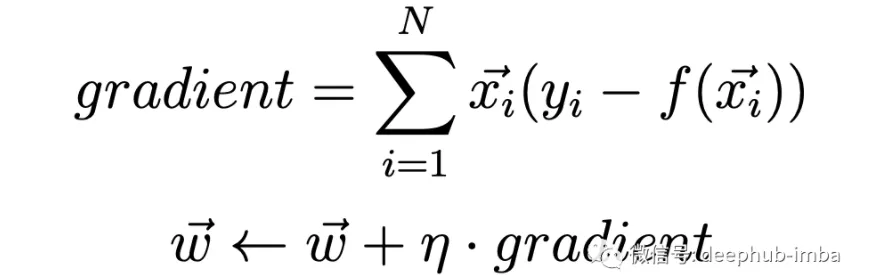
我们将使用此公式计算梯度。
在此,x(i)向量是一个点,其中N是数据集的大小。n(eta)是我们的学习率。y(i)向量是目标输出。f(x)向量是定义为f(x)= Sum(w * x)的回归线性函数,这里sum是sigma函数。另外,我们将考虑初始偏差w0 = 0并使得x0 =1。所有权重均初始化为0。
在此方法中,我们将平方误差总和用作损失函数。
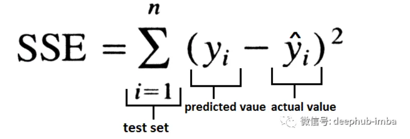
除了将SSE初始化为零外,我们将在每次迭代中记录SSE的变化,并将其与在程序执行之前提供的阈值进行比较。如果SSE低于阈值,程序将退出。
在该程序中,我们从命令行提供了三个输入。他们是:
threshold — 阈值,在算法终止之前,损失必须低于此阈值。
data — 数据集的位置。
learningRate — 梯度下降法的学习率。
因此,该程序的启动应该是这样的:
python3linearregr.py — datarandom.csv — learningRate 0.0001 — threshold 0.0001
在深入研究代码之前我们确定最后一件事,程序的输出将如下所示:
iteration_number,weight0,weight1,weight2,...,weightN,sum_of_squared_errors
该程序包括6个部分,我们逐个进行查看。
导入模块
import argparse # to read inputs from command lineimport csv # to read the input data set fileimport numpy as np # to work with the data set
初始化部分
# initialise argument parser and read argumentsfrom command line with the respective flags and then call the main() functionif __name__ == '__main__':
    parser = argparse.ArgumentParser()
    parser.add_argument("-d", "--data", help="Data File")
    parser.add_argument("-l", "--learningRate", help="Learning Rate")
    parser.add_argument("-t", "--threshold", help="Threshold")
    main()
main函数部分
defmain():
    args = parser.parse_args()
    file, learningRate, threshold = args.data, float(
        args.learningRate), float(args.threshold) # save respective command line inputs into variables# read csv file and the last column is the target output and is separated from the input (X) as Ywith open(file) as csvFile:
        reader = csv.reader(csvFile, delimiter=',')
        X = []
        Y = []
        for row in reader:
            X.append([1.0] + row[:-1])
            Y.append([row[-1]])
    # Convert data points into float and initialise weight vector with 0s.
    n = len(X)
    X = np.array(X).astype(float)
    Y = np.array(Y).astype(float)
    W = np.zeros(X.shape[1]).astype(float)
    # this matrix is transposed to match the necessary matrix dimensions for calculating dot product
    W = W.reshape(X.shape[1], 1).round(4)
    # Calculate the predicted output value
    f_x = calculatePredicatedValue(X, W)
    # Calculate the initial SSE
    sse_old = calculateSSE(Y, f_x)
    outputFile = 'solution_' + \
                 'learningRate_' + str(learningRate) + '_threshold_' \
                 + str(threshold) + '.csv''''
        Output file is opened in writing mode and the data is written in the format mentioned in the post. After the
        first values are written, the gradient and updated weights are calculated using the calculateGradient function.
        An iteration variable is maintained to keep track on the number of times the batch linear regression is executed
        before it falls below the threshold value. In the infinite while loop, the predicted output value is calculated
        again and new SSE value is calculated. If the absolute difference between the older(SSE from previous iteration)
        and newer(SSE from current iteration) SSE is greater than the threshold value, then above process is repeated.
        The iteration is incremented by 1 and the current SSE is stored into previous SSE. If the absolute difference
        between the older(SSE from previous iteration) and newer(SSE from current iteration) SSE falls below the
        threshold value, the loop breaks and the last output values are written to the file.
    '''with open(outputFile, 'w', newline='') as csvFile:
        writer = csv.writer(csvFile, delimiter=',', quoting=csv.QUOTE_NONE, escapechar='')
        writer.writerow([*[0], *["{0:.4f}".format(val) for val in W.T[0]], *["{0:.4f}".format(sse_old)]])
        gradient, W = calculateGradient(W, X, Y, f_x, learningRate)
        iteration = 1whileTrue:
            f_x = calculatePredicatedValue(X, W)
            sse_new = calculateSSE(Y, f_x)
            if abs(sse_new - sse_old) > threshold:
                writer.writerow([*[iteration], *["{0:.4f}".format(val) for val in W.T[0]], *["{0:.4f}".format(sse_new)]])
                gradient, W = calculateGradient(W, X, Y, f_x, learningRate)
                iteration += 1
                sse_old = sse_new
            else:
                break
        writer.writerow([*[iteration], *["{0:.4f}".format(val) for val in W.T[0]], *["{0:.4f}".format(sse_new)]])
    print("Output File Name: " + outputFile
main函数的流程如下所示:
- 将相应的命令行输入保存到变量中
- 读取CSV文件,最后一列是目标输出,与输入(存储为X)分开并存储为Y
- 将数据点转换为浮点初始化权重向量为0s
- 使用calculatePredicatedValue函数计算预测的输出值
- 使用calculateSSE函数计算初始SSE
- 输出文件以写入模式打开,数据以文章中提到的格式写入。写入第一个值后,使用calculateGradient函数计算梯度和更新的权重。进行变量迭代以确定线性回归在损失函数低于阈值之前执行的次数。在无限while循环中,再次计算预测的输出值,并计算新的SSE值。如果旧的(来自先前迭代的SSE)和较新的(来自当前迭代的SSE)之间的绝对差大于阈值,则重复上述过程。迭代次数增加1,当前SSE被存储到先前的SSE中。如果较旧的(上一次迭代的SSE)和较新的(当前迭代的SSE)之间的绝对差值低于阈值,则循环中断,并将最后的输出值写入文件。
calculatePredicatedValue函数
在此,通过执行输入矩阵X和权重矩阵W的点积来计算预测输出。
# dot product of X(input) and W(weights) as numpy matrices and returning the result which is the predicted outputdefcalculatePredicatedValue(X, W):
    f_x = np.dot(X, W)
    return f_x
calculateGradient函数
使用文章中提到的第一个公式计算梯度并更新权重。
defcalculateGradient(W, X, Y, f_x, learningRate):
    gradient = (Y - f_x) * X
    gradient = np.sum(gradient, axis=0)
    temp = np.array(learningRate * gradient).reshape(W.shape)
    W = W + temp
    return gradient, W
calculateSSE函数
使用上述公式计算SSE。
defcalculateSSE(Y, f_x):
    sse = np.sum(np.square(f_x - Y))
    return sse
现在,看完了完整的代码。让我们看一下程序的执行结果。

这是输出的样子:
00.00000.00000.00007475.31491-0.0940-0.5376-0.25922111.51052-0.1789-0.7849-0.3766880.69803-0.2555-0.8988-0.4296538.86384-0.3245-0.9514-0.4533399.80925-0.3867-0.9758-0.4637316.16826-0.4426-0.9872-0.4682254.51267-0.4930-0.9926-0.4699205.84798-0.5383-0.9952-0.4704166.69329-0.5791-0.9966-0.4704135.029310-0.6158-0.9973-0.4702109.389211-0.6489-0.9978-0.470088.619712-0.6786-0.9981-0.469771.794113-0.7054-0.9983-0.469458.163114-0.7295-0.9985-0.469147.120115-0.7512-0.9987-0.468938.173816-0.7708-0.9988-0.468730.926117-0.7883-0.9989-0.468525.054418-0.8042-0.9990-0.468320.297519-0.8184-0.9991-0.468116.443820-0.8312-0.9992-0.468013.321821-0.8427-0.9993-0.467810.792522-0.8531-0.9994-0.46778.743423-0.8625-0.9994-0.46767.083324-0.8709-0.9995-0.46755.738525-0.8785-0.9995-0.46744.649026-0.8853-0.9996-0.46743.766327-0.8914-0.9996-0.46733.051228-0.8969-0.9997-0.46722.471929-0.9019-0.9997-0.46722.002630-0.9064-0.9997-0.46711.622431-0.9104-0.9998-0.46711.314432-0.9140-0.9998-0.46701.064833-0.9173-0.9998-0.46700.862634-0.9202-0.9998-0.46700.698935-0.9229-0.9998-0.46690.566236-0.9252-0.9999-0.46690.458737-0.9274-0.9999-0.46690.371638-0.9293-0.9999-0.46690.301039-0.9310-0.9999-0.46680.243940-0.9326-0.9999-0.46680.197641-0.9340-0.9999-0.46680.160142-0.9353-0.9999-0.46680.129743-0.9364-0.9999-0.46680.105144-0.9374-0.9999-0.46680.085145-0.9384-0.9999-0.46680.069046-0.9392-0.9999-0.46680.055947-0.9399-1.0000-0.46670.045348-0.9406-1.0000-0.46670.036749-0.9412-1.0000-0.46670.029750-0.9418-1.0000-0.46670.024151-0.9423-1.0000-0.46670.019552-0.9427-1.0000-0.46670.015853-0.9431-1.0000-0.46670.012854-0.9434-1.0000-0.46670.010455-0.9438-1.0000-0.46670.008456-0.9441-1.0000-0.46670.006857-0.9443-1.0000-0.46670.005558-0.9446-1.0000-0.46670.004559-0.9448-1.0000-0.46670.003660-0.9450-1.0000-0.46670.002961-0.9451-1.0000-0.46670.002462-0.9453-1.0000-0.46670.001963-0.9454-1.0000-0.46670.001664-0.9455-1.0000-0.46670.001365-0.9457-1.0000-0.46670.001066-0.9458-1.0000-0.46670.000867-0.9458-1.0000-0.46670.000768-0.9459-1.0000-0.46670.000569-0.9460-1.0000-0.46670.000470-0.9461-1.0000-0.46670.0004
####最终程序
import argparse
import csv
import numpy as np
defmain():
    args = parser.parse_args()
    file, learningRate, threshold = args.data, float(
        args.learningRate), float(args.threshold) # save respective command line inputs into variables# read csv file and the last column is the target output and is separated from the input (X) as Ywith open(file) as csvFile:
        reader = csv.reader(csvFile, delimiter=',')
        X = []
        Y = []
        for row in reader:
            X.append([1.0] + row[:-1])
            Y.append([row[-1]])
    # Convert data points into float and initialise weight vector with 0s.
    n = len(X)
    X = np.array(X).astype(float)
    Y = np.array(Y).astype(float)
    W = np.zeros(X.shape[1]).astype(float)
    # this matrix is transposed to match the necessary matrix dimensions for calculating dot product
    W = W.reshape(X.shape[1], 1).round(4)
    # Calculate the predicted output value
    f_x = calculatePredicatedValue(X, W)
    # Calculate the initial SSE
    sse_old = calculateSSE(Y, f_x)
    outputFile = 'solution_' + \
                 'learningRate_' + str(learningRate) + '_threshold_' \
                 + str(threshold) + '.csv''''
        Output file is opened in writing mode and the data is written in the format mentioned in the post. After the
        first values are written, the gradient and updated weights are calculated using the calculateGradient function.
        An iteration variable is maintained to keep track on the number of times the batch linear regression is executed
        before it falls below the threshold value. In the infinite while loop, the predicted output value is calculated
        again and new SSE value is calculated. If the absolute difference between the older(SSE from previous iteration)
        and newer(SSE from current iteration) SSE is greater than the threshold value, then above process is repeated.
        The iteration is incremented by 1 and the current SSE is stored into previous SSE. If the absolute difference
        between the older(SSE from previous iteration) and newer(SSE from current iteration) SSE falls below the
        threshold value, the loop breaks and the last output values are written to the file.
    '''with open(outputFile, 'w', newline='') as csvFile:
        writer = csv.writer(csvFile, delimiter=',', quoting=csv.QUOTE_NONE, escapechar='')
        writer.writerow([*[0], *["{0:.4f}".format(val) for val in W.T[0]], *["{0:.4f}".format(sse_old)]])
        gradient, W = calculateGradient(W, X, Y, f_x, learningRate)
        iteration = 1whileTrue:
            f_x = calculatePredicatedValue(X, W)
            sse_new = calculateSSE(Y, f_x)
            if abs(sse_new - sse_old) > threshold:
                writer.writerow([*[iteration], *["{0:.4f}".format(val) for val in W.T[0]], *["{0:.4f}".format(sse_new)]])
                gradient, W = calculateGradient(W, X, Y, f_x, learningRate)
                iteration += 1
                sse_old = sse_new
            else:
                break
        writer.writerow([*[iteration], *["{0:.4f}".format(val) for val in W.T[0]], *["{0:.4f}".format(sse_new)]])
    print("Output File Name: " + outputFile
defcalculateGradient(W, X, Y, f_x, learningRate):
    gradient = (Y - f_x) * X
    gradient = np.sum(gradient, axis=0)
    # gradient = np.array([float("{0:.4f}".format(val)) for val in gradient])
    temp = np.array(learningRate * gradient).reshape(W.shape)
    W = W + temp
    return gradient, W
defcalculateSSE(Y, f_x):
    sse = np.sum(np.square(f_x - Y))
    return sse
defcalculatePredicatedValue(X, W):
    f_x = np.dot(X, W)
    return f_x
if __name__ == '__main__':
    parser = argparse.ArgumentParser()
    parser.add_argument("-d", "--data", help="Data File")
    parser.add_argument("-l", "--learningRate", help="Learning Rate")
    parser.add_argument("-t", "--threshold", help="Threshold")
    main()
这篇文章介绍了使用梯度下降法进行批线性回归的数学概念。在此,考虑了损失函数(在这种情况下为平方误差总和)。我们没有看到最小化SSE的方法,而这是不应该的(需要调整学习率),我们看到了如何在阈值的帮助下使线性回归收敛。
该程序使用numpy来处理数据,也可以使用python的基础知识而不使用numpy来完成,但是它将需要嵌套循环,因此时间复杂度将增加到O(n * n)。无论如何,numpy提供的数组和矩阵的内存效率更高。另外,如果您喜欢使用pandas模块,建议您使用它,并尝试使用它来实现相同的程序。
希望您喜欢这篇文章。谢谢阅读。