电子存储的医疗成像数据非常丰富，机器学习算法可以使用这种类型的数据集来检测和发现模式和异常。在本文中，我将向您介绍五个医疗保健领域的机器学习项目。

机器和算法可以解读成像数据，就像受过高度训练的放射科医生可以识别皮肤上的可疑斑点、病变、肿瘤和脑部出血一样。因此，机器学习工具和平台的使用，以帮助放射科医生准备增长指数。

机器学习被用于世界各地的许多领域。医疗保健行业也不例外。机器学习可以在预测运动障碍、心脏病、癌症、肺部疾病等方面发挥关键作用。

这些信息，如果提前很好地预测，可以为医生提供重要的信息，然后他们可以为每个患者量身定制诊断和治疗。现在让我们来看看一些医疗领域的机器学习项目。

心脏病预测：

心脏病描述了影响您心脏的一系列疾病。心脏疾病的疾病包括血管疾病，例如冠状动脉疾病，心律问题（心律不齐）和您天生的心脏缺陷（先天性心脏缺陷）等。

心脏病是世界人口发病率和死亡率的最大原因之一。在临床数据科学部分，心血管疾病的预测被认为是最重要的主题之一。医疗保健行业中的数据量巨大。

在这个数据科学项目中，我将应用机器学习技术对一个人是否患有心脏病进行分类。

`您可以从此处下载该项目所需的数据集：`

链接：https://pan.baidu.com/s/1aiXSnklK_q0BoaWhLLM2mQ

提取码：6rfj

导入所需的模块：

import numpy as np
import pandas as pd
import matplotlib.pyplot as plt
from matplotlib import rcParams
import seaborn as sns
import warnings
warnings.filterwarnings('ignore')

在这里，我们将使用KNeighborsClassifier进行实验：

from sklearn.neighbors import KNeighborsClassifier

现在让我们深入研究数据

df = pd.read_csv('dataset.csv')
print(df.head())

print(df.info())

输出

RangeIndex: 303 entries, 0 to 302
Data columns (total 14 columns):
age         303 non-null int64
sex         303 non-null int64
cp          303 non-null int64
trestbps    303 non-null int64
chol        303 non-null int64
fbs         303 non-null int64
restecg     303 non-null int64
thalach     303 non-null int64
exang       303 non-null int64
oldpeak     303 non-null float64
slope       303 non-null int64
ca          303 non-null int64
thal        303 non-null int64
target      303 non-null int64
dtypes: float64(1), int64(13)
memory usage: 33.2 KB

print(df.describe())

[外链图片转存失败,源站可能有防盗]!链机制,建(https://img-Wpblog.czdnimg.cn/imgonvert/a0ad52ecc264ca0e6473a29c790ee85e.png)]

特征选择

获取数据集中每个特征的相关性

import seaborn as sns
corrmat = df.corr()
top_corr_features = corrmat.index
plt.figure(figsize=(16,16))
#plot heat map
g=sns.heatmap(df[top_corr_features].corr(),annot=True,cmap="RdYlGn")
plt.show()

在目标类的大小大约相等的情况下，使用数据集始终是一个好习惯。因此，让我们检查一下是否相同：

sns.set_style('whitegrid')
sns.countplot(x='target',data=df,palette='RdBu_r')
plt.show()

数据处理

探索数据集后，我发现我需要在训练机器学习模型之前将一些分类变量转换为虚拟变量并缩放所有值。

首先，我将使用该 get_dummies 方法为分类变量创建虚拟列。

dataset = pd.get_dummies(df, columns = ['sex', 'cp', 
                                        'fbs','restecg', 
                                        'exang', 'slope', 
                                        'ca', 'thal'])
from sklearn.model_selection import train_test_split
from sklearn.preprocessing import StandardScaler
standardScaler = StandardScaler()
columns_to_scale = ['age', 'trestbps', 'chol', 'thalach', 'oldpeak']
dataset[columns_to_scale] = standardScaler.fit_transform(dataset[columns_to_scale])
dataset.head()

y = dataset['target']
X = dataset.drop(['target'], axis = 1)
from sklearn.model_selection import cross_val_score
knn_scores = []
for k in range(1,21):
    knn_classifier = KNeighborsClassifier(n_neighbors = k)
    score=cross_val_score(knn_classifier,X,y,cv=10)
    knn_scores.append(score.mean())
plt.plot([k for k in range(1, 21)], knn_scores, color = 'red')
for i in range(1,21):
    plt.text(i, knn_scores[i-1], (i, knn_scores[i-1]))
plt.xticks([i for i in range(1, 21)])
plt.xlabel('Number of Neighbors (K)')
plt.ylabel('Scores')
plt.title('K Neighbors Classifier scores for different K values')
plt.show()

knn_classifier = KNeighborsClassifier(n_neighbors = 12)
score=cross_val_score(knn_classifier,X,y,cv=10)
score.mean()

＃输出- 0.8448387096774195

随机森林分类器

from sklearn.ensemble import RandomForestClassifier
randomforest_classifier= RandomForestClassifier(n_estimators=10)
score=cross_val_score(randomforest_classifier,X,y,cv=10)
score.mean()

＃输出 - 0.8113978494623655

皮肤癌的分类:

皮肤癌是美国最常见的疾病之一。据报道，今年美国有多达400万人死于皮肤癌。在这里，您将学习如何使用机器学习创建皮肤癌分类模型。

这是一个巨大的数字，在一个国家就有400万人死于皮肤癌。就像所有这些死亡的人一样，但有一半甚至更多的病例，在疾病的早期没有去看医生而疾病本来是可以预防的。

皮肤癌是美国最常见的疾病之一。在过去的一年中，据报道有多达400万例死于皮肤癌的病例。在本文中，我将使用机器学习创建皮肤癌分类模型。

一个国家真的有400万人死于皮肤癌，这是一个巨大的数字。由于所有这些人都在死亡，但是其中一半甚至更多的病例在疾病可以预防的早期阶段就没有去看医生。

如果人们患上了皮肤癌的症状，他们仍然不愿意去看医生，这不是一个好信号，因为皮肤癌可以在早期阶段治愈。

机器学习对皮肤癌的分类

因此，这是机器学习算法在皮肤癌分类中起作用的地方。正如我之前提到的，皮肤癌可以在疾病的早期阶段很容易治愈，但这是人们不想去看医生的人。

因此，这是一个简单的机器学习算法，可以帮助那些人坐在家里时确定他们是否患有皮肤癌。该机器学习算法基于卷积神经网络（CNN）。

CNN层分类用于皮肤癌检测

让我们从导入库开始

import numpy as np
from skimage import io
import matplotlib.pyplot as plt

现在，我将简单地上传图像，以使用python中的skimage库来训练我们的机器学习模型。

imgb = io.imread('bimg-1049.png')
imgm = io.imread('mimg-178.png')
imgb = io.imread('bimg-721.png')
imgm = io.imread('mimg-57.png')

您可以从下面下载这些图像

链接：https://pan.baidu.com/s/17UB13G3NckDH4mXW7Bf25w

提取码：nh9p

这些图像是良性痣和恶性痣的样本图像，这是一种皮肤问题。

让我们展示这些图像

plt.figure(figsize=(10,20))
plt.subplot(121)
plt.imshow(imgb)
plt.axis('off')
plt.subplot(122)
plt.imshow(imgm)
plt.axis('off')

现在让我们训练模型以进行进一步分类

from keras.models import load_model
model = load_model('BM_VA_VGG_FULL_DA.hdf5')
from keras import backend as K
def activ_viewer(model, layer_name, im_put):
    layer_dict = dict([(layer.name, layer) for layer in model.layers])
    layer = layer_dict[layer_name]
    activ1 = K.function([model.layers[0].input, K.learning_phase()], [layer.output,])
    activations = activ1((im_put, False))
    return activations
def normalize(x):
    # utility function to normalize a tensor by its L2 norm
    return x / (K.sqrt(K.mean(K.square(x))) + 1e-5)
def deprocess_image(x):
    # normalize tensor: center on 0., ensure std is 0.1
    x -= x.mean()
    x /= (x.std() + 1e-5)
    x *= 0.1
    # clip to [0, 1]
    x += 0.5
    x = np.clip(x, 0, 1)
    # convert to RGB array
    x *= 255
    if K.image_data_format() == 'channels_first':
        x = x.transpose((1, 2, 0))
    x = np.clip(x, 0, 255).astype('uint8')
    return x
def plot_filters(filters):
    newimage = np.zeros((16*filters.shape[0],8*filters.shape[1]))
    for i in range(filters.shape[2]):
        y = i%8
        x = i//8
        newimage[x*filters.shape[0]:x*filters.shape[0]+filters.shape[0],
                 y*filters.shape[1]:y*filters.shape[1]+filters.shape[1]] = filters[:,:,i]
    plt.figure(figsize = (10,20))
    plt.imshow(newimage)
    plt.axis('off')

皮肤癌分类模型总结

要查看我们训练有素的模型的总结，我们将执行以下代码

model.summary()

_________________________________________________________________
Layer (type)                 Output Shape              Param #   
=================================================================
input_1 (InputLayer)         (None, 128, 128, 3)       0         
_________________________________________________________________
block1_conv1 (Conv2D)        (None, 128, 128, 64)      1792      
_________________________________________________________________
block1_conv2 (Conv2D)        (None, 128, 128, 64)      36928     
_________________________________________________________________
block1_pool (MaxPooling2D)   (None, 64, 64, 64)        0         
_________________________________________________________________
block2_conv1 (Conv2D)        (None, 64, 64, 128)       73856     
_________________________________________________________________
block2_conv2 (Conv2D)        (None, 64, 64, 128)       147584    
_________________________________________________________________
block2_pool (MaxPooling2D)   (None, 32, 32, 128)       0         
_________________________________________________________________
block3_conv1 (Conv2D)        (None, 32, 32, 256)       295168    
_________________________________________________________________
block3_conv2 (Conv2D)        (None, 32, 32, 256)       590080    
_________________________________________________________________
block3_conv3 (Conv2D)        (None, 32, 32, 256)       590080    
_________________________________________________________________
block3_pool (MaxPooling2D)   (None, 16, 16, 256)       0         
_________________________________________________________________
block4_conv1 (Conv2D)        (None, 16, 16, 512)       1180160   
_________________________________________________________________
block4_conv2 (Conv2D)        (None, 16, 16, 512)       2359808   
_________________________________________________________________
block4_conv3 (Conv2D)        (None, 16, 16, 512)       2359808   
_________________________________________________________________
block4_pool (MaxPooling2D)   (None, 8, 8, 512)         0         
_________________________________________________________________
block5_conv1 (Conv2D)        (None, 8, 8, 512)         2359808   
_________________________________________________________________
block5_conv2 (Conv2D)        (None, 8, 8, 512)         2359808   
_________________________________________________________________
block5_conv3 (Conv2D)        (None, 8, 8, 512)         2359808   
_________________________________________________________________
block5_pool (MaxPooling2D)   (None, 4, 4, 512)         0         
_________________________________________________________________
sequential_3 (Sequential)    (None, 1)                 2097665   
=================================================================
Total params: 16,812,353
Trainable params: 16,812,353
Non-trainable params: 0

现在让我们可视化我们训练过的模型的输出

activ_benign = activ_viewer(model,'block2_conv1',imgb.reshape(1,128,128,3))
img_benign = deprocess_image(activ_benign[0])
plot_filters(img_benign[0])
plt.figure(figsize=(20,20))
for f in range(128):
    plt.subplot(8,16,f+1)
    plt.imshow(img_benign[0,:,:,f])
    plt.axis('off')

现在让我们缩放和可视化一些过滤器

plt.figure(figsize=(10,10))
plt.subplot(121)
plt.imshow(img_benign[0,:,:,49])
plt.axis('off')
plt.subplot(122)
plt.imshow(img_malign[0,:,:,49])
plt.axis('off')

plt.figure(figsize=(10,10))
plt.subplot(121)
plt.imshow(img_benign[0,:,:,94])
plt.axis('off')
plt.subplot(122)
plt.imshow(img_malign[0,:,:,94])
plt.axis('off')

测试模型

现在让我们可视化并测试我们训练后的模型的实际能力

def plot_filters32(filters):
    newimage = np.zeros((16*filters.shape[0],16*filters.shape[1]))
    for i in range(filters.shape[2]):
        y = i%16
        x = i//16
        newimage[x*filters.shape[0]:x*filters.shape[0]+filters.shape[0],
                 y*filters.shape[1]:y*filters.shape[1]+filters.shape[1]] = filters[:,:,i]
    plt.figure(figsize = (15,25))
    plt.imshow(newimage)    
activ_benign = activ_viewer(model,'block3_conv3',imgb.reshape(1,128,128,3))
img_benign = deprocess_image(activ_benign[0])
plot_filters32(img_benign[0])

activ_malign = activ_viewer(model,'block3_conv3',imgm.reshape(1,128,128,3))
img_malign = deprocess_image(activ_malign[0])
plot_filters32(img_malign[0])

![](https://ucc.alicdn.com/images/user-upload-01/img_convert/33312643646f390c6e4374eb12931b08.png#align=left&display=inline&height=791&margin=[object Object]&originHeight=791&originWidth=800&size=0&status=done&style=none&width=800)

基于机器学习的肺分割:

肺分割是机器学习在医疗保健领域最有用的任务之一。肺CT图像分割是肺图像分析的一个必要的初始步骤，它是提供准确的肺CT图像分析如肺癌检测的初始步骤。

Dicom实际上是医学影像的存储库。这些文件包含大量元数据。这种分析的像素大小/粗度不同于不同的分析，这可能会对CNN方法的性能产生不利影响。

在本文中，我将向您介绍机器学习在医疗保健中的应用。我将向您展示如何使用python进行机器学习来完成肺分割任务。

肺分割是医疗保健中机器学习最有用的任务之一。肺部CT图像分割是进行肺部图像分析所必需的第一步，这是提供准确的肺部CT图像分析（例如检测肺癌）的初步步骤。

现在，让我们看看如何将机器学习用于肺部分割任务。在开始之前，我将导入一些软件包并确定可用的患者：

import numpy as np
import pandas as pd 
import dicom
import os
import scipy.ndimage
import matplotlib.pyplot as plt
from skimage import measure, morphology
from mpl_toolkits.mplot3d.art3d import Poly3DCollection
# Some constants 
INPUT_FOLDER = 'path to sample_images'
patients = os.listdir(INPUT_FOLDER)
patients.sort()

加载数据以进行肺分割

Dicom是医学成像中的事实上的存储库。这是我第一次使用它，但是看起来很简单。这些文件包含很多元数据。此分析像素大小/粗度因分析而异，这可能会对CNN方法的性能产生不利影响。

下面是加载分析的代码，其中包含多个切片，我们将它们简单地保存在Python列表中。数据集中的每个记录都是一个分析。缺少元数据字段，即Z方向上像素的大小，即切片的厚度。幸运的是，我们可以推断出它并将其添加到元数据中：

def load_scan(path):
    slices = [dicom.read_file(path + '/' + s) for s in os.listdir(path)]
    slices.sort(key = lambda x: float(x.ImagePositionPatient[2]))
    try:
        slice_thickness = np.abs(slices[0].ImagePositionPatient[2] - slices[1].ImagePositionPatient[2])
    except:
        slice_thickness = np.abs(slices[0].SliceLocation - slices[1].SliceLocation)
    for s in slices:
        s.SliceThickness = slice_thickness
    return slices

CT扫描的度量单位是Hounsfield单位（HU），它是放射密度的度量。CT扫描仪经过仔细校准，以准确地进行测量。

资料来源–维基百科

默认情况下，返回的值不在此单位中。我们首先需要解决此问题。

有些扫描仪有圆柱形扫描限制，但输出的图像是方形的。超出这些限制的像素得到固定值-2000。第一步是将这些值设置为0，即当前的air。然后回到HU单位，乘以调整后的斜率，再加上截距:

def get_pixels_hu(slices):
image = np.stack([s.pixel_array for s in slices])
# Convert to int16 (from sometimes int16),
# should be possible as values should always be low enough (<32k)
image = image.astype(np.int16)
# Set outside-of-scan pixels to 0
# The intercept is usually -1024, so air is approximately 0
image[image == -2000] = 0
# Convert to Hounsfield units (HU)
for slice_number in range(len(slices)):
    intercept = slices[slice_number].RescaleIntercept
    slope = slices[slice_number].RescaleSlope
    if slope != 1:
        image[slice_number] = slope * image[slice_number].astype(np.float64)
        image[slice_number] = image[slice_number].astype(np.int16)
    image[slice_number] += np.int16(intercept)
return np.array(image, dtype=np.int16)`

现在让我们看一下其中一名患者：

first_patient = load_scan(INPUT_FOLDER + patients[0])
first_patient_pixels = get_pixels_hu(first_patient)
plt.hist(first_patient_pixels.flatten(), bins=80, color='c')
plt.xlabel("Hounsfield Units (HU)")
plt.ylabel("Frequency")
plt.show()
# Show some slice in the middle
plt.imshow(first_patient_pixels[80], cmap=plt.cm.gray)
plt.show()

通过查看来自维基百科的肺部CT测量信息和上面的直方图，我们可以看到哪些像素是空气，哪些像素是组织。我们将在以后的肺分割任务中使用它。

重采样

CT扫描通常具有[2.5，0.5，0.5]的像素间距，这意味着切片之间的距离为2.5毫米。对于不同的分析，这可能是[1,5，0,725，0,725]，对于自动分析（例如，使用ConvNets）可能会出现问题。

解决此问题的一种常用方法是将整个数据集重新采样为特定的各向同性分辨率：

def resample(image, scan, new_spacing=[1,1,1]):
# Determine current pixel spacing
spacing = np.array([scan[0].SliceThickness] + scan[0].PixelSpacing, dtype=np.float32)
resize_factor = spacing / new_spacing
new_real_shape = image.shape * resize_factor
new_shape = np.round(new_real_shape)
real_resize_factor = new_shape / image.shape
new_spacing = spacing / real_resize_factor
image = scipy.ndimage.interpolation.zoom(image, real_resize_factor, mode='nearest')
return image, new_spacing`

当您将其应用于四舍五入的整个数据集时，这可能与所需的间距略有不同。我们需要将患者的像素重新采样到同构分辨率为1 x 1 x 1 mm：

pix_resampled, spacing = resample(first_patient_pixels, first_patient, [1,1,1])
print("Shape before resampling\t", first_patient_pixels.shape)
print("Shape after resampling\t", pix_resampled.shape)

Shape before resampling  (134, 512, 512)
Shape after resampling  (335, 306, 306)

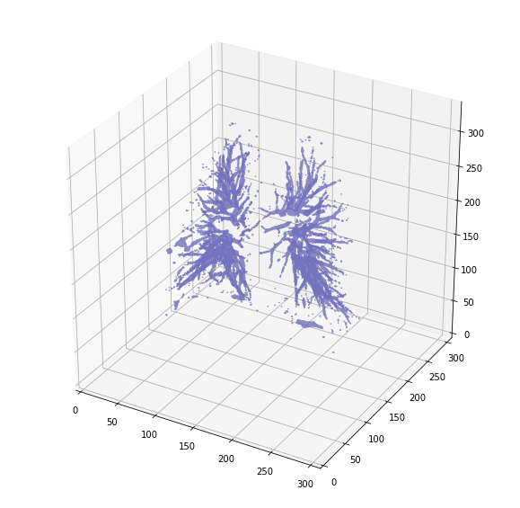
肺部3D绘图

对于可视化，能够显示扫描的3D图像是很有用的。所以我们将使用行走立方体为我们的3D对象创建一个粗略的网格，并使用matplotlib绘制:

``
def plot_3d(image, threshold=-300):
# Position the scan upright, 
# so the head of the patient would be at the top facing the camera
p = image.transpose(2,1,0)
verts, faces = measure.marching_cubes(p, threshold)
fig = plt.figure(figsize=(10, 10))
ax = fig.add_subplot(111, projection='3d')
# Fancy indexing: `verts[faces]` to generate a collection of triangles
mesh = Poly3DCollection(verts[faces], alpha=0.70)
face_color = [0.45, 0.45, 0.75]
mesh.set_facecolor(face_color)
ax.add_collection3d(mesh)
ax.set_xlim(0, p.shape[0])
ax.set_ylim(0, p.shape[1])
ax.set_zlim(0, p.shape[2])
plt.show()

我们的绘图函数采用一个参数，我们可以使用它来绘制结构，例如所有组织或仅骨骼。400是仅显示骨骼的良好阈值：

plot_3d(pix_resampled, 400)

肺分割

为了减少问题空间，我们可以分割肺部（通常是周围的某些组织）。我和我的同学们开发的方法非常有效。

它包括几个明智的步骤。它由一系列区域增长应用和形态操作组成。在这种情况下，我们将只使用连接组件的分析。

步骤：

图像阈值(-320 HU是一个很好的阈值，但无论如何这个方法)

制作连接组件，确定标签周围的空气，在二值图像中填充1s

可选:对于扫描的每一个轴向切片，确定最大的连接实体组件(身体+周围空气)，其余设置为0。这充满了面具的肺结构。

只保留最大的气囊(人体各处都有其他气囊)。

def largest_label_volume(im, bg=-1):
vals, counts = np.unique(im, return_counts=True)
counts = counts[vals != bg]
vals = vals[vals != bg]
if len(counts) &gt; 0:
return vals[np.argmax(counts)]
else:
return None
def segment_lung_mask(image, fill_lung_structures=True):
# not actually binary, but 1 and 2. 
# 0 is treated as background, which we do not want
binary_image = np.array(image &amp;gt; -320, dtype=np.int8)+1
labels = measure.label(binary_image)
# Pick the pixel in the very corner to determine which label is air.
#   Improvement: Pick multiple background labels from around the patient
#   More resistant to "trays" on which the patient lays cutting the air 
#   around the person in half
background_label = labels[0,0,0]
#Fill the air around the person
binary_image[background_label == labels] = 2
# Method of filling the lung structures (that is superior to something like 
# morphological closing)
if fill_lung_structures:
    # For every slice we determine the largest solid structure
    for i, axial_slice in enumerate(binary_image):
        axial_slice = axial_slice - 1
        labeling = measure.label(axial_slice)
        l_max = largest_label_volume(labeling, bg=0)
        if l_max is not None: #This slice contains some lung
            binary_image[i][labeling != l_max] = 1
binary_image -= 1 #Make the image actual binary
binary_image = 1-binary_image # Invert it, lungs are now 1
# Remove other air pockets insided body
labels = measure.label(binary_image, background=0)
l_max = largest_label_volume(labels, bg=0)
if l_max is not None: # There are air pockets
    binary_image[labels != l_max] = 0
return binary_image`

但有一件事我们可以解决，包括肺的结构(比如结节是固体的)可能是个好主意，我们不只是想在肺里通气:

segmented_lungs = segment_lung_mask(pix_resampled, False)
segmented_lungs_fill = segment_lung_mask(pix_resampled, True)
plot_3d(segmented_lungs, 0)

好多了让我们还可视化两者之间的区别：

plot_3d(segmented_lungs_fill - segmented_lungs, 0)

![](https://ucc.alicdn.com/images/user-upload-01/img_convert/35156ea694950a84fd7f6b0ac678903c.png#align=left&display=inline&height=565&margin=[object Object]&originHeight=565&originWidth=579&size=0&status=done&style=none&width=579)

希望您喜欢这篇关于肺分割的文章，将其作为机器学习在医疗保健中的应用。

预测糖尿病

根据美国疾病控制与预防中心(Centers for Disease Control and Prevention)的数据，目前约有七分之一的美国成年人患有糖尿病。但到2050年，这一比例将飙升至三分之一。考虑到这一点，我们将在这里学习:学习使用机器学习来帮助我们预测糖尿病。

让我们直接进入数据，您可以下载我在本文中使用的数据以预测以下糖尿病。

链接：https://pan.baidu.com/s/1j1f4q0Zb0p_l0U5vQ0Fjmg

提取码：2iot

import pandas as pd
import numpy as np
import matplotlib.pyplot as plt
%matplotlib inline
diabetes = pd.read_csv('diabetes.csv')
print(diabetes.columns)

Index(['Pregnancies', 'Glucose', 'BloodPressure', 
'SkinThickness', 'Insulin', 'BMI', 'DiabetesPedigreeFunction', 
'Age', 'Outcome'], dtype='object')

diabetes.head()

糖尿病数据集包含768个数据点，每个数据点有9个特征：

print("dimension of diabetes data: {}".format(diabetes.shape))

糖尿病数据的维度：（768，9）

“结果”是我们要预测的特征，0表示没有糖尿病，1表示糖尿病。在这768个数据点中，有500个被标记为0，而268被标记为1：

print(diabetes.groupby('Outcome').size())

import seaborn as sns sns.countplot(diabetes['Outcome'],label="Count")

diabetes.info()

K近邻可预测糖尿病

k最近邻居算法可以说是最简单的机器学习算法。建立模型仅包括存储训练数据集。为了对数据集中的新点进行预测，该算法在训练数据集中找到最接近的数据点-它的“最近邻居”。

首先，让我们研究是否可以确认模型复杂性和准确性之间的联系：

from sklearn.model_selection import train_test_split
X_train, X_test, y_train, y_test = train_test_split(diabetes.loc[:, diabetes.columns != 'Outcome'], diabetes['Outcome'], stratify=diabetes['Outcome'], random_state=66)
from sklearn.neighbors import KNeighborsClassifier
training_accuracy = []
test_accuracy = []
# try n_neighbors from 1 to 10
neighbors_settings = range(1, 11)
for n_neighbors in neighbors_settings:
    # build the model
    knn = KNeighborsClassifier(n_neighbors=n_neighbors)
    knn.fit(X_train, y_train)
    # record training set accuracy
    training_accuracy.append(knn.score(X_train, y_train))
    # record test set accuracy
    test_accuracy.append(knn.score(X_test, y_test))
plt.plot(neighbors_settings, training_accuracy, label="training accuracy")
plt.plot(neighbors_settings, test_accuracy, label="test accuracy")
plt.ylabel("Accuracy")
plt.xlabel("n_neighbors")
plt.legend()

让我们检查k近邻算法预测糖尿病的准确性得分。

knn = KNeighborsClassifier(n_neighbors=9)
knn.fit(X_train, y_train)
print('Accuracy of K-NN classifier on training set: {:.2f}'.format(knn.score(X_train, y_train)))
print('Accuracy of K-NN classifier on test set: {:.2f}'.format(knn.score(X_test, y_test)))

训练集上__的K-NN分类器的准确性_：0.79_

训练集上的K-NN分类器的准确性：0.78

决策树分类器

from sklearn.tree import DecisionTreeClassifier
tree = DecisionTreeClassifier(random_state=0)
tree.fit(X_train, y_train)
print("Accuracy on training set: {:.3f}".format(tree.score(X_train, y_train)))
print("Accuracy on test set: {:.3f}".format(tree.score(X_test, y_test)))

训练组的__准确性_：1.000_

测试组的准确性：0.714

使用决策树分类器的训练集的准确性为100％，而测试集的准确性则差得多。这表明树过度拟合并且不能很好地归纳为新数据。因此，我们需要对树进行预修剪。

现在，我将通过设置max_depth = 3再次执行此操作，限制树的深度可减少过度拟合。这会导致训练集的准确性降低，但会提高测试集的准确性。

tree = DecisionTreeClassifier(max_depth=3, random_state=0)
tree.fit(X_train, y_train)
print("Accuracy on training set: {:.3f}".format(tree.score(X_train, y_train)))
print("Accuracy on test set: {:.3f}".format(tree.score(X_test, y_test)))

训练组的__准确性_：0.773_

测试组的准确性：0.740

决策树中的特征重要性

功能重要性显示了每个功能对于决策树分类器做出的决策的重要性。对于每个功能，它是一个介于0和1之间的数字，其中0表示“完全不使用”，而1表示“完全预测目标”。功能重要性总和为1：

功能重要性：[0.04554275 0.6830362 0. 0. 0. 0.27142106 0. 0.]

现在让我们可视化决策树预测糖尿病的特征重要性。

def plot_feature_importances_diabetes(model):
    plt.figure(figsize=(8,6))
    n_features = 8
    plt.barh(range(n_features), model.feature_importances_, align='center')
    plt.yticks(np.arange(n_features), diabetes_features)
    plt.xlabel("Feature importance")
    plt.ylabel("Feature")
    plt.ylim(-1, n_features)
plot_feature_importances_diabetes(tree)

因此，葡萄糖功能最常用于预测糖尿病。

深度学习预测糖尿病

让我们训练一个深度学习模型来预测糖尿病：

from sklearn.neural_network import MLPClassifier
mlp = MLPClassifier(random_state=42)
mlp.fit(X_train, y_train)
print("Accuracy on training set: {:.2f}".format(mlp.score(X_train, y_train)))
print("Accuracy on test set: {:.2f}".format(mlp.score(X_test, y_test)))

_训练组的_准确性：0.71

测试组的准确性：0.67

多层感知器（MLP）的准确性根本不如其他模型，这可能是由于数据缩放所致。深度学习算法还期望所有输入特征以相似的方式变化，理想情况下，平均值为0，方差为1。现在，我将重新缩放我们的数据，以使其能够满足这些要求，从而以良好的准确性预测糖尿病。

from sklearn.preprocessing import StandardScaler
scaler = StandardScaler()
X_train_scaled = scaler.fit_transform(X_train)
X_test_scaled = scaler.fit_transform(X_test)
mlp = MLPClassifier(random_state=0)
mlp.fit(X_train_scaled, y_train)
print("Accuracy on training set: {:.3f}".format(
    mlp.score(X_train_scaled, y_train)))
print("Accuracy on test set: {:.3f}".format(mlp.score(X_test_scaled, y_test)))

_训练集的_准确性：0.823

测试集的准确性：0.802

现在，我们增加迭代次数，alpha参数，并为模型的权重添加更强的参数：

mlp = MLPClassifier(max_iter=1000, alpha=1, random_state=0)
mlp.fit(X_train_scaled, y_train)
print("Accuracy on training set: {:.3f}".format(
    mlp.score(X_train_scaled, y_train)))
print("Accuracy on test set: {:.3f}".format(mlp.score(X_test_scaled, y_test))

_训练组的_准确性：0.795

测试组的准确性：0.792

结果很好，但是我们无法进一步提高测试精度。因此，到目前为止，我们最好的模型是缩放后的默认深度学习模型。现在，我将在上学习的神经网络中绘制第一层权重的热图，以使用数据集预测糖尿病。

plt.figure(figsize=(20, 5))
plt.imshow(mlp.coefs_[0], interpolation='none', cmap='viridis')
plt.yticks(range(8), diabetes_features)
plt.xlabel("Columns in weight matrix")
plt.ylabel("Input feature")
plt.colorbar()

新冠病毒接触者追踪:

联系人跟踪如何工作？

一旦一个人的冠状病毒呈阳性，确定可能已被诊断出的患者感染的其他人非常重要。为了确定感染者，当局会追踪最近14天诊断出的患者的活动。此过程称为联系人跟踪。根据国家和地方当局，可以通过手动方法或数字方法来进行联系搜索。

在本文中，我将提出一种依赖GPS数据的数字接触跟踪算法，该算法可用于机器学习的接触跟踪。

机器学习中的联系人跟踪

DBSCAN是基于密度的数据聚类算法，可对给定空间中的数据点进行分组。DBSCAN算法将彼此靠近的数据点分组，并将离群的数据点标记为噪声。我将使用DBSCAN算法来进行机器学习中的联系人跟踪任务。

我将在此任务中使用的数据集是JSON数据，可以下载。现在，让我们导入此任务所需的所有库，并开始阅读数据集并从数据中探索一些见解：

链接：https://pan.baidu.com/s/1VOiKlSdmIGtZdZabVY1MNg

提取码：xji7

import numpy as np
import pandas as pd
import matplotlib.pyplot as plt
import seaborn as sns
%matplotlib inline
import datetime as dt
from sklearn.cluster import DBSCAN
df = pd.read_json(‘livedata.json’)
df.head()

现在，让我们使用散点图分析数据集，该散点图显示id分别在x轴和Y轴上的经度和纬度：

plt.figure(figsize=(8,6))
sns.scatterplot(x=‘latitude’, y=‘longitude’, data=df, hue=‘id’)
plt.legend(bbox_to_anchor= [1, 0.8])

使用机器学习为联系人跟踪创建模型

现在，让我们使用DBSCAN模型创建一个用于联系人跟踪的模型。下面的函数将帮助我们创建DBSCAN模型，使用该模型我们将生成集群，该集群将通过过滤集群中的数据来帮助识别感染：

def get_infected_names(input_name):
    epsilon = 0.0018288 # a radial distance of 6 feet in kilometers
    model = DBSCAN(eps=epsilon, min_samples=2, metric='haversine').fit(df[['latitude', 'longitude']])
    df['cluster'] = model.labels_.tolist()
    input_name_clusters = []
    for i in range(len(df)):
        if df['id'][i] == input_name:
            if df['cluster'][i] in input_name_clusters:
                pass
            else:
                input_name_clusters.append(df['cluster'][i])
    infected_names = []
    for cluster in input_name_clusters:
        if cluster != -1:
            ids_in_cluster = df.loc[df['cluster'] == cluster, 'id']
            for i in range(len(ids_in_cluster)):
                member_id = ids_in_cluster.iloc[i]
                if (member_id not in infected_names) and (member_id != input_name):
                    infected_names.append(member_id)
                else:
                    pass
    return infected_names

现在，让我们使用我们的模型生成集群

epsilon = 0.0018288 # a radial distance of 6 feet in kilometers
model = DBSCAN(eps=epsilon, min_samples=1, metric='haversine').fit(df[['latitude', 'longitude']])
labels = model.labels_
fig = plt.figure(figsize=(12,10))
sns.scatterplot(df['latitude'], df['longitude'], hue = ['cluster-{}'.format(x) for x in labels])
plt.legend(bbox_to_anchor = [1, 1])
plt.show()

追踪感染者

要查找可能被患者感染的人，我们只需调用get_infected_names函数并输入数据集中的名称作为参数：

print(get_infected_names("Erin"))

手把手教你用python实现机器学习预测疾病

心脏病预测：

`您可以从此处下载该项目所需的数据集：`

现在让我们深入研究数据

特征选择

数据处理

随机森林分类器

皮肤癌的分类:

机器学习对皮肤癌的分类

CNN层分类用于皮肤癌检测

皮肤癌分类模型总结

测试模型

基于机器学习的肺分割:

加载数据以进行肺分割

重采样

肺部3D绘图

肺分割

预测糖尿病

K近邻可预测糖尿病

决策树分类器

决策树中的特征重要性

深度学习预测糖尿病

新冠病毒接触者追踪:

联系人跟踪如何工作？

机器学习中的联系人跟踪

使用机器学习为联系人跟踪创建模型

追踪感染者

热门文章

最新文章

相关课程

相关电子书

相关实验场景

推荐镜像

热门

活动广场

任务中心

开发者评测

高校计划

乘风者计划

训练营

阿里云MVP

话题

直播

下载

镜像站

技术资料

插件

手把手教你用python实现机器学习预测疾病

心脏病预测：

您可以从此处下载该项目所需的数据集：

现在让我们深入研究数据

特征选择

数据处理

随机森林分类器

皮肤癌的分类:

机器学习对皮肤癌的分类

CNN层分类用于皮肤癌检测

皮肤癌分类模型总结

测试模型

基于机器学习的肺分割:

加载数据以进行肺分割

重采样

肺部3D绘图

肺分割

预测糖尿病

K近邻可预测糖尿病

决策树分类器

决策树中的特征重要性

深度学习预测糖尿病

新冠病毒接触者追踪:

联系人跟踪如何工作？

机器学习中的联系人跟踪

使用机器学习为联系人跟踪创建模型

追踪感染者

热门文章

最新文章

相关课程

相关电子书

相关实验场景

推荐镜像

`您可以从此处下载该项目所需的数据集：`