目录
Designing Network Design Spaces
3.1. Tools for Design Space Design 设计空间设计工具
3.2. The AnyNet Design Space AnyNet的设计空间
3.3. The RegNet Design Space RegNet设计空间
3.4. Design Space Generalization 设计空间泛化
4. Analyzing the RegNetX Design Space 分析RegNetX设计空间
5. Comparison to Existing Networks 与现有网络的比较
5.1. State-of-the-Art Comparison: Mobile Regime 最先进的比较:移动系统
5.2. Standard Baselines Comparison: ResNe(X)t 标准基线比较:ResNe(X)t
5.3. State-of-the-Art Comparison: Full Regime 最先进的比较:完全制度
论文地址:https://arxiv.org/pdf/2003.13678.pdf
Designing Network Design Spaces
Abstract 摘要
| In this work, we present a new network design paradigm. Our goal is to help advance the understanding of network design and discover design principles that generalize across settings. Instead of focusing on designing individual network instances, we design network design spaces that parametrize populations of networks. The overall process is analogous to classic manual design of networks, but elevated to the design space level. Using our methodology we explore the structure aspect of network design and arrive at a low-dimensional design space consisting of simple, regular networks that we call RegNet. The core insight of the RegNet parametrization is surprisingly simple: widths and depths of good networks can be explained by a quantized linear function. We analyze the RegNet design space and arrive at interesting findings that do not match the current practice of network design. The RegNet design space provides simple and fast networks that work well across a wide range of flop regimes. Under comparable training settings and flops, the RegNet models outperform the popular EfficientNet models while being up to 5× faster on GPUs. | 在这项工作中,我们提出了一个新的网络设计范例。我们的目标是帮助提高对网络设计的理解,并发现跨设置泛化的设计原则。我们不是专注于设计单个的网络实例,而是设计参数化网络总体的网络设计空间。整个过程类似于经典的手工网络设计,但是提升到了设计空间的层次。使用我们的方法,我们探索了网络设计的结构方面,并得出一个由简单的、规则的网络组成的低维设计空间,我们称之为RegNet。RegNet参数化的核心思想非常简单:良好网络的宽度和深度可以用量化的线性函数来解释。我们分析了RegNet设计空间,得出了与当前网络设计实践不相符的有趣发现。RegNet设计空间提供了简单而快速的网络,可以很好地跨越各种触发器。在可比较的训练设置和flops的情况下,RegNet模型在gpu上的运行速度高达5倍,表现优于当前流行的有效网模型。 |
1. Introduction 介绍
| Deep convolutional neural networks are the engine of visual recognition. Over the past several years better architectures have resulted in considerable progress in a wide range of visual recognition tasks. Examples include LeNet [15], AlexNet [13], VGG [26], and ResNet [8]. This body of work advanced both the effectiveness of neural networks as well as our understanding of network design. In particular, the above sequence of works demonstrated the importance of convolution, network and data size, depth, and residuals, respectively. The outcome of these works is not just particular network instantiations, but also design principles that can be generalized and applied to numerous settings. | 深度卷积神经网络是视觉识别的引擎。在过去的几年里,更好的体系结构在视觉识别领域取得了长足的进步。例如LeNet[15]、AlexNet[13]、VGG[26]和ResNet[8]。这一工作体系既提高了神经网络的有效性,也提高了我们对网络设计的理解。特别是上述工作序列,分别说明了卷积、网络和数据大小、深度和残差的重要性。这些工作的结果不仅是特定的网络实例化,而且是设计原则,可以推广和应用于许多设置。 |
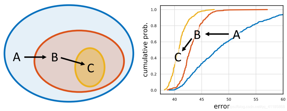
Figure 1. Design space design. We propose to design network design spaces, where a design space is a parametrized set of possible model architectures. Design space design is akin to manual network design, but elevated to the population level. In each step of our process the input is an initial design space and the output is a refined design space of simpler or better models. Following [21], we characterize the quality of a design space by sampling models and inspecting their error distribution. For example, in the figure above we start with an initial design space A and apply two refinement steps to yield design spaces B then C. In this case C ⊆ B ⊆A (left), and the error distributions are strictly improving from A to B to C (right). The hope is that design principles that apply to model populations are more likely to be robust and generalize. While manual network design has led to large advances, finding well-optimized networks manually can be challenging, especially as the number of design choices increases. A popular approach to address this limitation is neural architecture search (NAS). Given a fixed search space of possible networks, NAS automatically finds a good model within the search space. Recently, NAS has received a lot of attention and shown excellent results [34, 18, 29]. Despite the effectiveness of NAS, the paradigm has limitations. The outcome of the search is a single network instance tuned to a specific setting (e.g., hardware platform). This is sufficient in some cases; however, it does not enable discovery of network design principles that deepen our understanding and allow us to generalize to new settings. In particular, our aim is to find simple models that are easy to understand, build upon, and generalize. |
图1所示。设计空间设计。我们建议设计网络设计空间,其中设计空间是可能的模型架构的参数化集合。设计空间设计类似于人工网络设计,但提升到了人口层面。在我们流程的每个步骤中,输入是初始设计空间,输出是更简单或更好模型的精细化设计空间。在[21]之后,我们通过采样模型并检查它们的误差分布来描述设计空间的质量。例如,在上图中我们从最初的设计空间和应用两个改进措施产量设计空间B C。在这种情况下C⊆B⊆(左),和误差分布严格改善从A到B C(右)。希望适用于模型总体的设计原则更有可能是健壮的和一般化的。 虽然手动网络设计已经取得了很大的进展,但是手动找到优化良好的网络可能是一项挑战,特别是在设计选择的数量增加的情况下。解决这一限制的一种流行方法是神经架构搜索(NAS)。给定一个可能的网络的固定搜索空间,NAS会自动在搜索空间中找到一个好的模型。近年来,NAS受到了广泛的关注,并取得了良好的研究成果[34,18,29]。 尽管NAS有效,但这种范式也有局限性。搜索的结果是将单个网络实例调优到特定的设置(例如,硬件平台)。在某些情况下,这就足够了;然而,它并不能帮助我们发现网络设计原则,从而加深我们的理解,并使我们能够归纳出新的设置。特别是,我们的目标是找到易于理解、构建和泛化的简单模型。 |
In this work, we present a new network design paradigm that combines the advantages of manual design and NAS. Instead of focusing on designing individual network instances, we design design spaces that parametrize populations of networks.1 Like in manual design, we aim for interpretability and to discover general design principles that describe networks that are simple, work well, and generalize across settings. Like in NAS, we aim to take advantage of semi-automated procedures to help achieve these goals. The general strategy we adopt is to progressively design simplified versions of an initial, relatively unconstrained, design space while maintaining or improving its quality (Figure 1). The overall process is analogous to manual design, elevated to the population level and guided via distribution estimates of network design spaces [21]. As a testbed for this paradigm, our focus is on exploring network structure (e.g., width, depth, groups, etc.) assuming standard model families including VGG [26], ResNet [8], and ResNeXt [31]. We start with a relatively unconstrained design space we call AnyNet (e.g., widths and depths vary freely across stages) and apply our humanin-the-loop methodology to arrive at a low-dimensional design space consisting of simple “regular” networks, that we call RegNet. The core of the RegNet design space is simple: stage widths and depths are determined by a quantized linear function. Compared to AnyNet, the RegNet design space has simpler models, is easier to interpret, and has a higher concentration of good models. |
在这项工作中,我们提出了一个新的网络设计范例,它结合了手工设计和NAS的优点。我们不是专注于设计单个的网络实例,而是设计参数化网络总体的设计空间。和手工设计一样,我们的目标是可解释性,并发现描述网络的一般设计原则,这些网络简单、工作良好,并且可以在各种设置中泛化。与NAS一样,我们的目标是利用半自动过程来帮助实现这些目标。 我们采用的一般策略是逐步设计一个初始的、相对不受约束的设计空间的简化版本,同时保持或提高其质量(图1)。整个过程类似于手工设计,提升到总体水平,并通过网络设计空间[21]的分布估计进行指导。 作为这个范例的一个测试平台,我们的重点是探索假定标准模型族包括VGG[26]、ResNet[8]和ResNeXt[31]的网络结构(例如,宽度、深度、组等)。我们从一个相对不受约束的设计空间开始,我们称之为AnyNet(例如,宽度和深度在不同阶段自由变化),并应用我们的人在循环的方法来达到一个由简单的“规则”网络组成的低维设计空间,我们称之为RegNet。RegNet设计空间的核心很简单:舞台宽度和深度由量化的线性函数决定。与AnyNet相比,RegNet设计空间具有更简单的模型,更易于解释,并且具有更高的优秀模型集中度。
|
We design the RegNet design space in a low-compute, low-epoch regime using a single network block type on ImageNet [3]. We then show that the RegNet design space generalizes to larger compute regimes, schedule lengths, and network block types. Furthermore, an important property of the design space design is that it is more interpretable and can lead to insights that we can learn from. We analyze the RegNet design space and arrive at interesting findings that do not match the current practice of network design. For example, we find that the depth of the best models is stable across compute regimes (∼20 blocks) and that the best models do not use either a bottleneck or inverted bottleneck. We compare top REGNET models to existing networks in various settings. First, REGNET models are surprisingly effective in the mobile regime. We hope that these simple models can serve as strong baselines for future work. Next, REGNET models lead to considerable improvements over standard RESNE(X)T [8, 31] models in all metrics. We highlight the improvements for fixed activations, which is of high practical interest as the number of activations can strongly influence the runtime on accelerators such as GPUs. Next, we compare to the state-of-the-art EFFICIENTNET [29] models across compute regimes. Under comparable training settings and flops, REGNET models outperform EFFICIENTNET models while being up to 5× faster on GPUs. We further test generalization on ImageNetV2 [24]. We note that network structure is arguably the simplest form of a design space design one can consider. Focusing on designing richer design spaces (e.g., including operators) may lead to better networks. Nevertheless, the structure will likely remain a core component of such design spaces. In order to facilitate future research we will release all code and pretrained models introduced in this work.2 |
我们使用ImageNet[3]上的单一网络块类型,在低计算、低历元的情况下设计了RegNet设计空间。然后,我们展示了RegNet设计空间可以泛化为更大的计算状态、调度长度和网络块类型。此外,设计空间设计的一个重要特性是,它具有更强的可解释性,并能带来我们可以学习的见解。我们分析了RegNet设计空间,得出了与当前网络设计实践不相符的有趣发现。例如,我们发现最佳模型的深度在不同的计算机制(∼20块)之间是稳定的,并且最佳模型既不使用瓶颈,也不使用反向瓶颈。 我们将顶级的REGNET模型与各种环境下的现有网络进行比较。首先,REGNET模型在移动环境中非常有效。我们希望这些简单的模型可以作为未来工作的强大基线。接下来,REGNET模型在所有指标上都比标准的RESNE(X)T[8,31]模型有了显著的改进。我们强调了对固定激活的改进,这是一个很有实际意义的问题,因为激活的数量会对加速程序(如gpu)的运行时间产生很大的影响。接下来,我们比较最先进的高效网络[29]模型的计算制度。在可比较的训练设置和失败的情况下,REGNET模型比有效的net模型表现得更好,同时在gpu上可以达到5倍的速度。我们进一步测试了在ImageNetV2[24]上的泛化。 我们注意到,网络结构可以说是人们可以考虑的最简单的设计空间形式。专注于设计更丰富的设计空间(例如,包括运营商)可能会导致更好的网络。然而,该结构可能仍然是此类设计空间的核心组成部分。 为了方便未来的研究,我们将发布所有的代码和在此工作中引入的预训练模型 |
2. Related Work 相关工作
Manual network design. The introduction of AlexNet [13] catapulted network design into a thriving research area. In the following years, improved network designs were proposed; examples include VGG [26], Inception [27, 28], ResNet [8], ResNeXt [31], DenseNet [11], and MobileNet [9, 25]. The design process behind these networks was largely manual and focussed on discovering new design choices that improve accuracy e.g., the use of deeper models or residuals. We likewise share the goal of discovering new design principles. In fact, our methodology is analogous to manual design but performed at the design space level. Automated network design. Recently, the network design process has shifted from a manual exploration to more automated network design, popularized by NAS. NAS has proven to be an effective tool for finding good models, e.g., [35, 23, 17, 20, 18, 29]. The majority of work in NAS focuses on the search algorithm, i.e., efficiently finding the best network instances within a fixed, manually designed search space (which we call a design space). Instead, our focus is on a paradigm for designing novel design spaces. The two are complementary: better design spaces can improve the efficiency of NAS search algorithms and also lead to existence of better models by enriching the design space. |
手动网络设计。AlexNet[13]的引入使网络设计成为一个蓬勃发展的研究领域。在接下来的几年里,提出了改进的网络设计;例如VGG [26], Inception [27,28], ResNet [8], ResNeXt [31], DenseNet[11],和MobileNet[9,25]。这些网络背后的设计过程很大程度上是手工的,并且专注于发现新的设计选择,以提高准确性,例如使用更深层次的模型或残差。我们同样分享发现新设计原则的目标。事实上,我们的方法类似于手工设计,但是在设计空间级别执行。 自动化的网络设计。最近,网络设计的过程已经从手工探索转向了自动化程度更高的网络设计,并由NAS推广开来。NAS已被证明是寻找良好模型的有效工具,如[35,23,17,20,18,29]。NAS的大部分工作集中在搜索算法上,即,在一个固定的、手工设计的搜索空间(我们称之为设计空间)中高效地找到最佳网络实例。相反,我们关注的是设计新颖设计空间的范例。两者是相辅相成的:更好的设计空间可以提高NAS搜索算法的效率,并且通过丰富设计空间来产生更好的模型。 |
Network scaling. Both manual and semi-automated network design typically focus on finding best-performing network instances for a specific regime (e.g., number of flops comparable to ResNet-50). Since the result of this procedure is a single network instance, it is not clear how to adapt the instance to a different regime (e.g., fewer flops). A common practice is to apply network scaling rules, such as varying network depth [8], width [32], resolution [9], or all three jointly [29]. Instead, our goal is to discover general design principles that hold across regimes and allow for efficient tuning for the optimal network in any target regime. Comparing networks. Given the vast number of possible network design spaces, it is essential to use a reliable comparison metric to guide our design process. Recently, the authors of [21] proposed a methodology for comparing and analyzing populations of networks sampled from a design space. This distribution-level view is fully-aligned with our goal of finding general design principles. Thus, we adopt this methodology and demonstrate that it can serve as a useful tool for the design space design process. |
网络扩展。手动和半自动网络设计通常都关注于为特定的机制寻找性能最佳的网络实例(例如,与ResNet-50相当的失败数)。由于这个过程的结果是一个单一的网络实例,所以不清楚如何使实例适应不同的机制(例如,更少的失败)。一种常见的做法是应用网络缩放规则,如改变网络深度[8]、宽度[32]、分辨率[9]或三者同时改变[29]。相反,我们的目标是发现普遍的设计原则,这些原则适用于各种制度,并允许对任何目标制度下的最佳网络进行有效的调优。 比较网络。考虑到大量可能的网络设计空间,使用可靠的比较度量来指导我们的设计过程是至关重要的。最近,[21]的作者提出了一种比较和分析从设计空间中采样的网络总体的方法。这个分布级视图与我们寻找通用设计原则的目标完全一致。因此,我们采用这种方法,并证明它可以作为一个有用的工具,为设计空间的设计过程。 |
| Parameterization. Our final quantized linear parameterization shares similarity with previous work, e.g. how stage widths are set [26, 7, 32, 11, 9]. However, there are two key differences. First, we provide an empirical study justifying the design choices we make. Second, we give insights into structural design choices that were not previously understood (e.g., how to set the number of blocks in each stages). | 参数化。我们最终的量化线性参数化与之前的工作有相似之处,例如如何设置舞台宽度[26,7,32,11,9]。然而,有两个关键的区别。首先,我们提供了一个实证研究证明我们所做的设计选择。其次,我们提供了以前不了解的结构设计选择(例如,如何在每个阶段设置块的数量)。 |
3. Design Space Design 设计空间设计
Our goal is to design better networks for visual recognition. Rather than designing or searching for a single best model under specific settings, we study the behavior of populations of models. We aim to discover general design principles that can apply to and improve an entire model population. Such design principles can provide insights into network design and are more likely to generalize to new settings (unlike a single model tuned for a specific scenario). We rely on the concept of network design spaces introduced by Radosavovic et al. [21]. A design space is a large, possibly infinite, population of model architectures. The core insight from [21] is that we can sample models from a design space, giving rise to a model distribution, and turn to tools from classical statistics to analyze the design space. We note that this differs from architecture search, where the goal is to find the single best model from the space. |
我们的目标是设计更好的视觉识别网络。我们不是在特定的环境下设计或寻找单一的最佳模型,而是研究模型总体的行为。我们的目标是发现一般的设计原则,可以适用于和改善整个模型人口。这样的设计原则可以提供对网络设计的洞察,并且更有可能泛化到新的设置中(不同于针对特定场景进行调整的单个模型)。 我们依靠Radosavovic等人提出的网络设计空间的概念。一个设计空间是一个庞大的,可能是无限的,模型架构的种群。[21]的核心观点是,我们可以从设计空间中抽取模型样本,生成模型分布,并使用经典统计数据中的工具来分析设计空间。我们注意到这与架构搜索不同,架构搜索的目标是从空间中找到单个的最佳模型。 |
In this work, we propose to design progressively simplified versions of an initial, unconstrained design space. We refer to this process as design space design. Design space design is akin to sequential manual network design, but elevated to the population level. Specifically, in each step of our design process the input is an initial design space and the output is a refined design space, where the aim of each design step is to discover design principles that yield populations of simpler or better performing models. We begin by describing the basic tools we use for design space design in §3.1. Next, in §3.2 we apply our methodology to a design space, called AnyNet, that allows unconstrained network structures. In §3.3, after a sequence of design steps, we obtain a simplified design space consisting of only regular network structures that we name RegNet. Finally, as our goal is not to design a design space for a single setting, but rather to discover general principles of network design that generalize to new settings, in §3.4 we test the generalization of the RegNet design space to new settings. Relative to the AnyNet design space, the RegNet design space is: (1) simplified both in terms of its dimension and type of network configurations it permits, (2) contains a higher concentration of top-performing models, and (3) is more amenable to analysis and interpretation. |
在这项工作中,我们建议设计一个逐步简化版本的初始,无约束的设计空间。我们将这个过程称为设计空间设计。设计空间设计类似于顺序的手工网络设计,但提升到总体水平。具体地说,在我们的设计过程的每一步中,输入是一个初始设计空间,输出是一个精细化的设计空间,其中每一步的目的是发现设计原则,从而生成更简单或性能更好的模型。 我们首先在§3.1中描述我们用于设计空间设计的基本工具。接下来,在§3.2中,我们将我们的方法应用于一个称为AnyNet的设计空间,该设计空间允许无约束的网络结构。在§3.3中,经过一系列设计步骤之后,我们获得了一个简化的设计空间,该空间只由我们命名为RegNet的规则网络结构组成。最后,由于我们的目标不是为单个设置设计一个设计空间,而是发现网络设计的一般原则,这些原则可以推广到新的设置,在§3.4中,我们测试了RegNet设计空间推广到新的设置的情况。 相对于AnyNet设计空间,RegNet设计空间是:(1)在它所允许的网络配置的尺寸和类型方面都进行了简化;(2)包含了更集中的性能最好的模型;(3)更易于分析和解释。 |
3.1. Tools for Design Space Design 设计空间设计工具
| We begin with an overview of tools for design space design. To evaluate and compare design spaces, we use the tools introduced by Radosavovic et al. [21], who propose to quantify the quality of a design space by sampling a set of models from that design space and characterizing the resulting model error distribution. The key intuition behind this approach is that comparing distributions is more robust and informative than using search (manual or automated) and comparing the best found models from two design spaces. | 我们首先概述用于设计空间设计的工具。为了评估和比较设计空间,我们使用了Radosavovic等人提出的工具,他们提出通过从设计空间中抽取一组模型并对结果模型误差分布进行表征来量化设计空间的质量。这种方法背后的主要直觉是,与使用搜索(手动或自动)和比较来自两个设计空间的最佳模型相比,比较发行版更健壮、更有信息性。 |
Figure 2. Statistics of the AnyNetX design space computed with n = 500 sampled models. Left: The error empirical distribution function (EDF) serves as our foundational tool for visualizing the quality of the design space. In the legend we report the min error and mean error (which corresponds to the area under the curve). Middle: Distribution of network depth d (number of blocks) versus error. Right: Distribution of block widths in the fourth stage (w4) versus error. The blue shaded regions are ranges containing the best models with 95% confidence (obtained using an empirical bootstrap), and the black vertical line the most likely best value. |
图2。使用n = 500个采样模型计算AnyNetX设计空间的统计信息。左:误差经验分布函数(EDF)是我们可视化设计空间质量的基本工具。在图例中,我们报告了最小误差和平均误差(对应于曲线下的面积)。中间:网络深度d(块数)与错误的分布。右:块宽在第四阶段(w4)的分布与误差。蓝色阴影区域是包含95%置信度的最佳模型的范围(使用经验自助法获得),而黑色竖线是最有可能的最佳值。 |
To obtain a distribution of models, we sample and train n models from a design space. For efficiency, we primarily do so in a low-compute, low-epoch training regime. In particular, in this section we use the 400 million flop3 (400MF) regime and train each sampled model for 10 epochs on the ImageNet dataset [3]. We note that while we train many models, each training run is fast: training 100 models at 400MF for 10 epochs is roughly equivalent in flops to training a single ResNet-50 [8] model at 4GF for 100 epochs. As in [21], our primary tool for analyzing design space quality is the error empirical distribution function (EDF). The error EDF of n models with errors ei is given by: F(e) gives the fraction of models with error less than e. We show the error EDF for n = 500 sampled models from the AnyNetX design space (described in §3.2) in Figure 2 (left). |
为了获得模型的分布,我们从一个设计空间中采样并训练n个模型。为了提高效率,我们主要在低计算、低时代的训练体制下进行。特别地,在本节中,我们使用4亿个flop3 (400MF)机制,并在ImageNet数据集[3]上对每个采样模型进行10个纪元的训练。我们注意到,虽然我们训练了许多模型,但每一次训练都是快速的:在400MF下训练100个模型10个epoch与在4GF下训练单个ResNet-50[8]模型100 epoch大致相当。 与[21]一样,我们分析设计空间质量的主要工具是误差经验分布函数(EDF)。有误差ei的n个模型的误差EDF为: F(e)给出了误差小于e的模型的比例。我们在图2(左)中展示了来自AnyNetX设计空间(在§3.2中描述)的n = 500个采样模型的误差EDF。 |
Given a population of trained models, we can plot and analyze various network properties versus network error, see Figure 2 (middle) and (right) for two examples taken from the AnyNetX design space. Such visualizations show 1D projections of a complex, high-dimensional space, and can help obtain insights into the design space. For these plots, we employ an empirical bootstrap4 [5] to estimate the likely range in which the best models fall. To summarize: (1) we generate distributions of models obtained by sampling and training n models from a design space, (2) we compute and plot error EDFs to summarize design space quality, (3) we visualize various properties of a design space and use an empirical bootstrap to gain insight, and (4) we use these insights to refine the design space. |
给定一组训练过的模型,我们可以绘制和分析各种网络属性与网络错误之间的关系,参见图2(中间)和图2(右边),这两个示例取自AnyNetX设计空间。这样的可视化显示了一个复杂的高维空间的一维投影,可以帮助获得对设计空间的洞察。对于这些图,我们使用一个经验bootstrap4[5]来估计最佳模型的可能范围。 总结:(1)我们生成分布模型获得的采样和训练n模型的设计空间,(2)我们计算和绘制错误edf总结设计空间质量,(3)我们想象的各种属性设计空间和使用经验引导了解,(4),我们使用这些信息来改进设计空间。
|
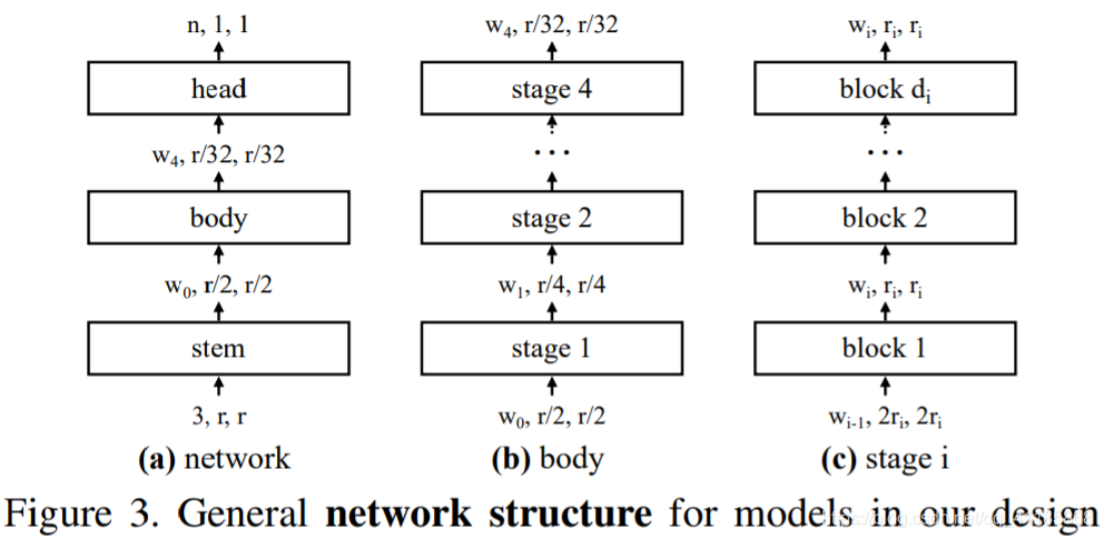
Figure 3. General network structure for models in our design spaces. (a) Each network consists of a stem (stride-two 3×3 conv with w0 = 32 output channels), followed by the network body that performs the bulk of the computation, and then a head (average pooling followed by a fully connected layer) that predicts n output classes. (b) The network body is composed of a sequence of stages that operate at progressively reduced resolution ri. (c) Each stage consists of a sequence of identical blocks, except the first block which uses stride-two conv. While the general structure is simple, the total number of possible network configurations is vast. |
图3。我们设计空间中模型的一般网络结构。(a)每个网络包括一个stem (stride-two 3×3 conv with w0 = 32 output channels),接着是执行大部分计算的网络主体,然后是预测n个输出类的head(平均池接全连接层)。(b)网络主体由一系列按逐步降低分辨率ri操作的阶段组成。(c)除了第一个使用stride-two conv的块外,每个阶段都由一系列相同的块组成。虽然一般结构简单,但可能的网络配置的总数是巨大的。 |
3.2. The AnyNet Design Space AnyNet的设计空间
We next introduce our initial AnyNet design space. Our focus is on exploring the structure of neural networks assuming standard, fixed network blocks (e.g., residual bottleneck blocks). In our terminology the structure of the network includes elements such as the number of blocks (i.e. network depth), block widths (i.e. number of channels), and other block parameters such as bottleneck ratios or group widths. The structure of the network determines the distribution of compute, parameters, and memory throughout the computational graph of the network and is key in determining its accuracy and efficiency. The basic design of networks in our AnyNet design space is straightforward. Given an input image, a network consists of a simple stem, followed by the network body that performs the bulk of the computation, and a final network head that predicts the output classes, see Figure 3a. We keep the stem and head fixed and as simple as possible, and instead focus on the structure of the network body that is central in determining network compute and accuracy. |
接下来,我们将介绍我们最初的AnyNet设计空间。我们的重点是探索假定标准的固定网络块(例如,剩余瓶颈块)的神经网络结构。在我们的术语中,网络的结构包括一些元素,如块的数量(即网络深度)、块的宽度(即通道的数量)和其他块的参数(如瓶颈比率或组的宽度)。网络的结构决定了计算、参数和内存在整个网络计算图中的分布,是决定其准确性和效率的关键。 在我们的AnyNet设计空间中,网络的基本设计非常简单。给定一个输入图像,一个网络由一个简单的主干、执行大部分计算的网络主体和预测输出类的最终网络头组成,如图3a所示。我们保持杆和头固定,尽可能简单,相反,我们关注网络主体的结构,这是决定网络计算和精度的核心。 |
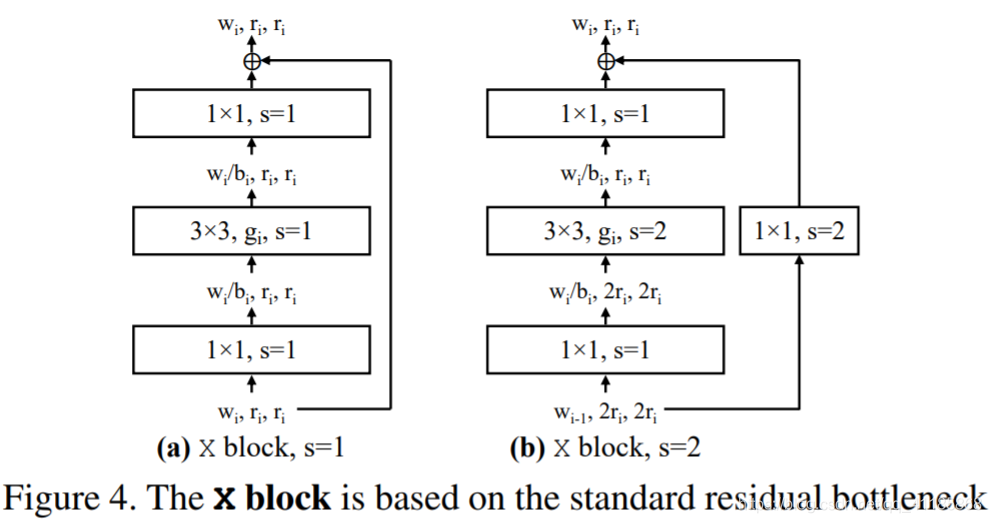
Figure 4. The X block is based on the standard residual bottleneck block with group convolution [31]. (a) Each X block consists of a 1×1 conv, a 3×3 group conv, and a final 1×1 conv, where the 1×1 convs alter the channel width. BatchNorm [12] and ReLU follow each conv. The block has 3 parameters: the width wi, bottleneck ratio bi, and group width gi. (b) The stride-two (s = 2) version. |
图4。X块基于标准剩余瓶颈块,组卷积为[31]。(a)每个X块由一个1×1 conv、一个3×3 group conv和一个最终的1×1 conv组成,其中1×1 convs改变通道宽度。BatchNorm[12]和ReLU遵循每个conv, block有3个参数:宽度wi,瓶颈比bi,组宽度gi。(b)第二版(s = 2)。 网络主体由4个阶段组成,以逐渐降低的分辨率运行,参见图3b(我们在§3.4中探讨了阶段数量的变化)。每个阶段由一系列相同的块组成,参见图3c。总的来说,对于每个阶段i,自由度包括块的数量di、块宽度wi和任何其他块参数。虽然总体结构很简单,但AnyNet设计空间中可能存在的网络总数是巨大的。 |
The network body consists of 4 stages operating at progressively reduced resolution, see Figure 3b (we explore varying the number of stages in §3.4). Each stage consists of a sequence of identical blocks, see Figure 3c. In total, for each stage i the degrees of freedom include the number of blocks di , block width wi , and any other block parameters. While the general structure is simple, the total number of possible networks in the AnyNet design space is vast. Most of our experiments use the standard residual bottlenecks block with group convolution [31], shown in Figure 4. We refer to this as the X block, and the AnyNet design space built on it as AnyNetX (we explore other blocks in §3.4). While the X block is quite rudimentary, we show it can be surprisingly effective when network structure is optimized. The AnyNetX design space has 16 degrees of freedom as each network consists of 4 stages and each stage i has 4 parameters: the number of blocks di , block width wi , bottleneck ratio bi , and group width gi . We fix the input resolution r = 224 unless otherwise noted. To obtain valid models, we perform log-uniform sampling of di ≤ 16, wi ≤ 1024 and divisible by 8, bi ∈ {1, 2, 4}, and gi ∈ {1, 2, . . . , 32} (we test these ranges later). We repeat the sampling until we obtain n = 500 models in our target complexity regime (360MF to 400MF), and train each model for 10 epochs.5 Basic statistics for AnyNetX were shown in Figure 2. |
我们的实验大多使用标准的残差瓶颈块与组卷积[31],如图4所示。我们将其称为X块,在其上构建的AnyNet设计空间称为AnyNetX(我们将在§3.4中讨论其他块)。虽然X块非常简陋,但我们证明了它在优化网络结构时可以非常有效。 AnyNetX设计空间有16个自由度,因为每个网络由4个阶段组成,每个阶段i有4个参数:块数量di、块宽度wi、瓶颈比bi和组宽度gi。我们修正了输入分辨率r = 224,除非另有说明。为了得到有效的模型,我们对di≤16,wi≤1024,且可被8整除,bi∈{1,2,4},gi∈{1,2,…, 32}(稍后测试这些范围)。我们重复采样,直到在我们的目标复杂度范围内(360 - 400MF)获得n = 500个模型,并对每个模型进行10个epoch的训练。AnyNetX的基本统计数据如图2所示。 |
sic statistics for AnyNetX were shown in Figure 2. There are (16·128·3·6)4 ≈ 1018 possible model configurations in the AnyNetX design space. Rather than searching for the single best model out of these ∼1018 configurations, we explore whether there are general design principles that can help us understand and refine this design space. To do so, we apply our approach of designing design spaces. In each step of this approach, our aims are:
|
AnyNetX的sic统计数据如图2所示。在AnyNetX设计空间中有(16·128·3·6)4≈1018种可能的模型配置。我们不是从这些∼1018配置中寻找单个的最佳模型,而是探究是否有通用的设计原则可以帮助我们理解和改进这个设计空间。为此,我们采用了设计设计空间的方法。在这方法的每一步,我们的目标是:
|
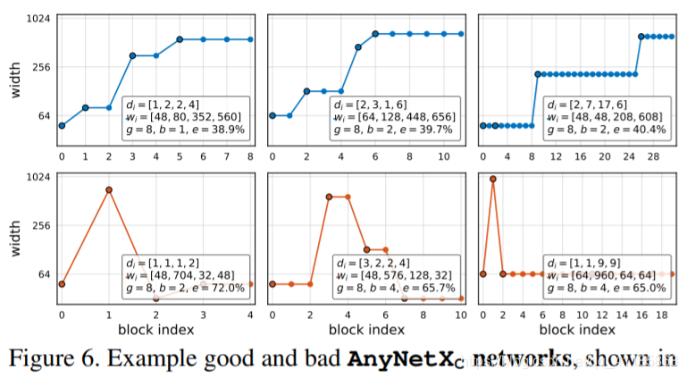
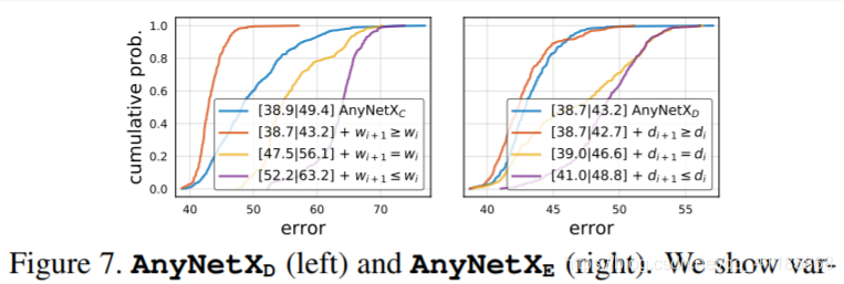
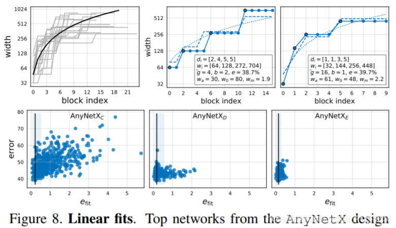
Figure 5. AnyNetXB (left) and AnyNetXC (middle) introduce a shared bottleneck ratio bi = b and shared group width gi = g, respectively. This simplifies the design spaces while resulting in virtually no change in the error EDFs. Moreover, AnyNetXB and AnyNetXC are more amendable to analysis. Applying an empirical bootstrap to b and g we see trends emerge, e.g., with 95% confidence b ≤ 2 is best in this regime (right). No such trends are evident in the individual bi and gi in AnyNetXA (not shown). Figure 6. Example good and bad AnyNetXC networks, shown in the top and bottom rows, respectively. For each network, we plot the width wj of every block j up to the network depth d. These per-block widths wj are computed from the per-stage block depths di and block widths wi (listed in the legends for reference). Figure 7. AnyNetXD (left) and AnyNetXE (right). We show various constraints on the per stage widths wi and depths di. In both cases, having increasing wi and di is beneficial, while using constant or decreasing values is much worse. Note that AnyNetXD = AnyNetXC + wi+1 ≥ wi, and AnyNetXE = AnyNetXD + di+1 ≥ di. We explore stronger constraints on wi and di shortly. Figure 8. Linear fits. Top networks from the AnyNetX design space can be well modeled by a quantized linear parameterization, and conversely, networks for which this parameterization has a higher fitting error efit tend to perform poorly. See text for details. |
图5。AnyNetXB(左)和AnyNetXC(中)分别引入了共享瓶颈比bi = b和共享组宽度gi = g。这简化了设计空间,同时几乎不会改变错误EDFs。此外,AnyNetXB和AnyNetXC更易于进行分析。对b和g应用经验自举法,我们可以看到趋势的出现,例如,在这种情况下,95%置信b≤2是最好的(右)。在AnyNetXA的个体bi和gi中没有明显的这种趋势(未显示)。
图6。示例好的和坏的AnyNetXC网络,分别显示在顶部和底部行。对于每个网络,我们绘制每个块j的宽度wj,直到网络深度d。这些每个块宽度wj是由每个阶段的块深度di和块宽度wi计算出来的(列在图例中以供参考)。
图7。AnyNetXD(左)和AnyNetXE(右)。我们给出了每个阶段宽度wi和深度di的各种约束条件。在这两种情况下,增加wi和di是有益的,而使用常数或递减值则更糟。注意AnyNetXD = AnyNetXC + wi+1≥wi,且AnyNetXE = AnyNetXD + di+1≥di。我们将很快探讨对wi和di的更强约束。 |
We now apply this approach to the AnyNetX design space. AnyNetXA. For clarity, going forward we refer to the initial, unconstrained AnyNetX design space as AnyNetXA. AnyNetXB. We first test a shared bottleneck ratio bi = b for all stages i for the AnyNetXA design space, and refer to the resulting design space as AnyNetXB. As before, we sample and train 500 models from AnyNetXB in the same settings. The EDFs of AnyNetXA and AnyNetXB, shown in Figure 5 (left), are virtually identical both in the average and best case. This indicates no loss in accuracy when coupling the bi . In addition to being simpler, the AnyNetXB is more amenable to analysis, see for example Figure 5 (right). AnyNetXC. Our second refinement step closely follows the first. Starting with AnyNetXB, we additionally use a shared group width gi = g for all stages to obtain AnyNetXC. As before, the EDFs are nearly unchanged, see Figure 5 (middle). Overall, AnyNetXC has 6 fewer degrees of freedom than AnyNetXA, and reduces the design space size nearly four orders of magnitude. Interestingly, we find g > 1 is best (not shown); we analyze this in more detail in §4. AnyNetXD. Next, we examine typical network structures of both good and bad networks from AnyNetXC in Figure 6. A pattern emerges: good network have increasing widths. We test the design principle of wi+1 ≥ wi , and refer to the design space with this constraint as AnyNetXD. In Figure 7 (left) we see this improves the EDF substantially. We return to examining other options for controlling width shortly. AnyNetXE. Upon further inspection of many models (not shown), we observed another interesting trend. In addition to stage widths wi increasing with i, the stage depths di likewise tend to increase for the best models, although not necessarily in the last stage. Nevertheless, we test a design space variant AnyNetXE with di+1 ≥ di in Figure 7 (right), and see it also improves results. Finally, we note that the constraints on wi and di each reduce the design space by 4!, with a cumulative reduction of O(107 ) from AnyNetXA. |
我们现在将这种方法应用于AnyNetX设计空间。AnyNetXA。为了清晰起见,我们将最初的、不受约束的AnyNetX设计空间称为AnyNetXA。AnyNetXB。我们首先测试AnyNetXA设计空间的所有阶段i的共享瓶颈比bi = b,并将得到的设计空间称为AnyNetXB。与之前一样,我们在相同的设置下从AnyNetXB取样和培训了500个模型。如图5(左)所示,AnyNetXA和AnyNetXB的edf在平均情况和最佳情况下实际上是相同的。这表示在耦合bi时没有精度损失。除了更简单之外,AnyNetXB更易于分析,参见图5(右侧)。 AnyNetXC。我们的第二个细化步骤紧跟着第一个步骤。从AnyNetXB开始,我们还为所有阶段使用共享的组宽度gi = g来获得AnyNetXC。与前面一样,EDFs几乎没有变化,请参见图5(中间)。总的来说,AnyNetXC比AnyNetXA少了6个自由度,并且减少了近4个数量级的设计空间大小。有趣的是,我们发现g > 1是最好的(没有显示);我们将在§4中对此进行更详细的分析。AnyNetXD。接下来,我们将研究图6中AnyNetXC中好的和坏的网络的典型网络结构。一种模式出现了:良好的网络具有不断增长的宽度。我们测试了wi+1≥wi的设计原则,并将此约束下的设计空间称为AnyNetXD。在图7(左)中,我们看到这极大地改进了EDF。稍后我们将讨论控制宽度的其他选项。AnyNetXE。在进一步检查许多模型(未显示)后,我们观察到另一个有趣的趋势。除了阶段宽度wi随i增加外,对于最佳模型,阶段深度di也同样趋向于增加,尽管不一定是在最后阶段。尽管如此,在图7(右)中,我们测试了一个设计空间变体AnyNetXE,其中di+1≥di,并看到它也改善了结果。最后,我们注意到对wi和di的约束使设计空间减少了4!,与AnyNetXA相比O(107)的累积减少。 |
3.3. The RegNet Design Space RegNet设计空间
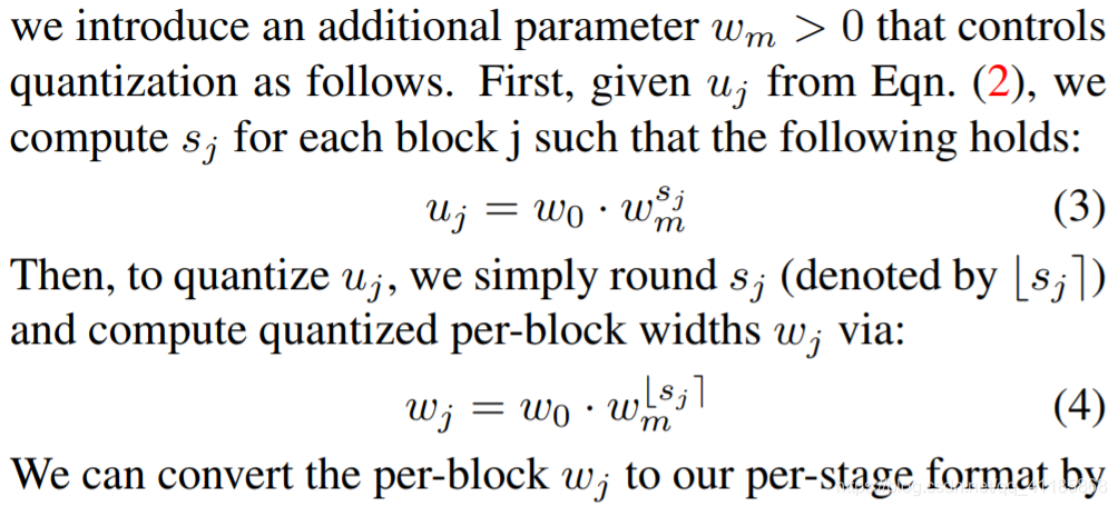
To gain further insight into the model structure, we show the best 20 models from AnyNetXE in a single plot, see Figure 8 (top-left). For each model, we plot the per-block width wj of every block j up to the network depth d (we use i and j to index over stages and blocks, respectively). See Figure 6 for reference of our model visualization. While there is significant variance in the individual models (gray curves), in the aggregate a pattern emerges. In particular, in the same plot we show the line wj = 48·(j+1)for 0 ≤ j ≤ 20 (solid black curve, please note that the y-axis is logarithmic). Remarkably, this trivial linear fit seems to explain the population trend of the growth of network widths for top models. Note, however, that this linear fit assigns a different width wj to each block, whereas individual models have quantized widths (piecewise constant functions). To see if a similar pattern applies to individual models, we need a strategy to quantize a line to a piecewise constant function. Inspired by our observations from AnyNetXD and AnyNetXE, we propose the following approach. First, we introduce a linear parameterization for block widths: This parameterization has three parameters: depth d, initial width w0 > 0, and slope wa > 0, and generates a different block width uj for each block j < d. To quantize uj , We can convert the per-block wj to our per-stage format by simply counting the number of blocks with constant width, that is, each stage i has block width wi = w0·w i m and number of blocks di = P j 1[bsj e = i]. When only considering four stage networks, we ignore the parameter combinations that give rise to a different number of stages. |
为了进一步了解模型结构,我们在一个图中显示了来自AnyNetXE的最好的20个模型,见图8(左上)。对于每个模型,我们绘制每个块j的每块宽度wj,直到网络深度d(我们分别使用i和j来索引阶段和块)。请参阅图6,以了解我们的模型可视化。 虽然在个别模型(灰色曲线)中存在显著的差异,但在总体上出现了一种模式。特别地,在相同的图中,我们显示了0≤j≤20时的wj = 48·(j+1)(实心黑色曲线,请注意y轴是对数的)。值得注意的是,这种琐碎的线性拟合似乎可以解释顶级模型网络宽度增长的总体趋势。然而,请注意,这个线性拟合为每个块分配了不同的宽度wj,而单个模型具有量化的宽度(分段常数函数)。 要查看类似的模式是否适用于单个模型,我们需要一种策略来将一条线量化为分段常数函数。受AnyNetXD和AnyNetXE的启发,我们提出了以下方法。首先,我们引入一个块宽的线性参数化: 该参数化有三个参数:深度d、初始宽度w0 >和斜率wa > 0,并为每个区块j < d生成不同的区块宽度uj。为了量化uj, 我们可以将每个块的wj转换为我们的每个阶段的格式,只需计算具有恒定宽度的块的数量,即每个阶段i的块宽度wi = w0·w im,块数量di = P j 1[bsj e = i]。当只考虑四个阶段网络时,我们忽略了引起不同阶段数的参数组合。 图9。RegNetX设计空间。详情见正文。 |
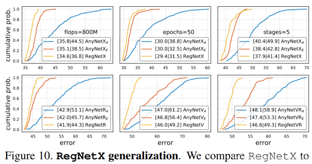
Figure 9. RegNetX design space. See text for details. Figure 10. RegNetX generalization. We compare RegNetX to AnyNetX at higher flops (top-left), higher epochs (top-middle), with 5-stage networks (top-right), and with various block types (bottom). In all cases the ordering of the design spaces is consistent and we see no signs of design space overfitting. Table 1. Design space summary. See text for details. |
图10。RegNetX泛化。我们比较了RegNetX和AnyNetX在更高的flops(左上)、更高的epoch(中上)、5级网络(右上)和各种块类型(下)的性能。在所有情况下,设计空间的顺序是一致的,我们没有看到设计空间过拟合的迹象。 表1。设计空间的总结。详情见正文。
|
We test this parameterization by fitting to models from AnyNetX. In particular, given a model, we compute the fit by setting d to the network depth and performing a grid search over w0, wa and wm to minimize the mean log-ratio (denoted by efit) of predicted to observed per-block widths. Results for two top networks from AnyNetXE are shown in Figure 8 (top-right). The quantized linear fits (dashed curves) are good fits of these best models (solid curves). Next, we plot the fitting error efit versus network error for every network in AnyNetXC through AnyNetXE in Figure 8 (bottom). First, we note that the best models in each design space all have good linear fits. Indeed, an empirical bootstrap gives a narrow band of efit near 0 that likely contains the best models in each design space. Second, we note that on average, efit improves going from AnyNetXC to AnyNetXE, showing that the linear parametrization naturally enforces related constraints to wi and di increasing. To further test the linear parameterization, we design a design space that only contains models with such linear structure. In particular, we specify a network structure via 6 parameters: d, w0, wa, wm (and also b, g). Given these, we generate block widths and depths via Eqn. (2)-(4). We refer to the resulting design space as RegNet, as it contains only simple, regular models. We sample d < 64, w0, wa < 256, 1.5 ≤ wm ≤ 3 and b and g as before (ranges set based on efit on AnyNetXE). |
我们通过拟合来自AnyNetX的模型来测试这个参数化。特别地,在给定的模型中,我们通过设置网络深度d并在w0、wa和wm上执行网格搜索来计算拟合,从而最小化每个块宽度的预测与观察的平均日志比(用efit表示)。来自AnyNetXE的两个顶级网络的结果如图8所示(右上角)。量化的线性拟合(虚线)是这些最佳模型(实线)的良好拟合。 接下来,我们通过AnyNetXE绘制AnyNetXC中每个网络的拟合错误efit与网络错误,如图8(底部)所示。首先,我们注意到每个设计空间中最好的模型都具有良好的线性拟合。实际上,经验引导法给出了一个接近于0的efit窄频带,它可能包含每个设计空间中最好的模型。其次,我们注意到efit从AnyNetXC到AnyNetXE的平均性能得到了改善,这表明线性参数化自然地对wi和di的增加施加了相关的约束。 为了进一步检验线性参数化,我们设计了一个只包含线性结构模型的设计空间。特别地,我们通过6个参数来指定网络结构:d, w0, wa, wm(以及b, g),给定这些参数,我们通过Eqn来生成块的宽度和深度。(2)- (4)。我们将最终的设计空间称为RegNet,因为它只包含简单的、常规的模型。我们对d < 64、w0、wa < 256、1.5≤wm≤3和b、g进行采样(根据AnyNetXE上的efit设置范围)。 |
The error EDF of RegNetX is shown in Figure 9 (left). Models in RegNetX have better average error than AnyNetX while maintaining the best models. In Figure 9 (middle) we test two further simplifications. First, using wm = 2 (doubling width between stages) slightly improves the EDF, but we note that using wm ≥ 2 performs better (shown later). Second, we test setting w0 = wa, further simplifying the linear parameterization to uj = wa ·(j + 1). Interestingly, this performs even better. However, to maintain the diversity of models, we do not impose either restriction. Finally, in Figure 9 (right) we show that random search efficiency is much higher for RegNetX; searching over just ∼32 random models is likely to yield good models. Table 1 shows a summary of the design space sizes (for RegNet we estimate the size by quantizing its continuous parameters). In designing RegNetX, we reduced the dimension of the original AnyNetX design space from 16 to 6 dimensions, and the size nearly 10 orders of magnitude. We note, however, that RegNet still contains a good diversity of models that can be tuned for a variety of settings. |
我们通过拟合来自AnyNetX的模型来测试这个参数化。特别地,在给定的模型中,我们通过设置网络深度d并在w0,佤邦和wm上执行网格搜索来计算拟合,从而最小化每个块宽度的预测与观察的平均日志比(用efit表示)。来自AnyNetXE的两个顶级网络的结果如图8所示(右上角)。量化的线性拟合(虚线)是这些最佳模型(实线)的良好拟合。 图9(左)显示了RegNetX的EDF错误。在维护最佳模型的同时,RegNetX中的模型具有比AnyNetX更好的平均错误。在图9(中间)中,我们测试了两个进一步的简化。首先,使用wm = 2(两个阶段之间的宽度加倍)稍微提高了EDF,但是我们注意到使用wm≥2性能更好(稍后将展示)。其次,我们测试设置w0 = wa,进一步将线性参数化简化为uj = wa·(j + 1),有趣的是,这样做的效果更好。然而,为了保持模型的多样性,我们不施加任何限制。最后,在图9(右)中,我们展示了RegNetX的随机搜索效率要高得多;只对∼32随机模型进行搜索可能会得到好的模型。 表1显示了设计空间大小的摘要(对于RegNet,我们通过量化其连续参数来估计大小)。在设计RegNetX时,我们将原始AnyNetX设计空间的维度从16个维度缩减为6个维度,大小接近10个数量级。但是,我们注意到,RegNet仍然包含各种各样的模型,可以针对各种设置进行调优。 |
3.4. Design Space Generalization 设计空间泛化
We designed the RegNet design space in a low-compute, low-epoch training regime with only a single block type. However, our goal is not to design a design space for a single setting, but rather to discover general principles of network design that can generalize to new settings. In Figure 10, we compare the RegNetX design space to AnyNetXA and AnyNetXE at higher flops, higher epochs, with 5-stage networks, and with various block types (described in the appendix). In all cases the ordering of the design spaces is consistent, with RegNetX > AnyNetXE > AnyNetXA. In other words, we see no signs of overfitting. These results are promising because they show RegNet can generalize to new settings. The 5-stage results show the regular structure of RegNet can generalize to more stages, where AnyNetXA has even more degrees of freedom. |
我们在只有一个块类型的低计算、低历元训练机制中设计了RegNet设计空间。然而,我们的目标不是为单一的设置设计一个设计空间,而是发现可以推广到新设置的网络设计的一般原则。 在图10中,我们将RegNetX设计空间与AnyNetXA和AnyNetXE在更高的flops、更高的epoch、5级网络和各种块类型(在附录中进行了描述)下进行了比较。在所有情况下,设计空间的顺序是一致的,使用RegNetX > AnyNetXE > AnyNetXA。换句话说,我们没有看到过度拟合的迹象。这些结果很有希望,因为它们表明RegNet可以泛化到新的设置。5阶段的结果表明,正则RegNet结构可以推广到更多的阶段,其中AnyNetXA具有更多的自由度。 |
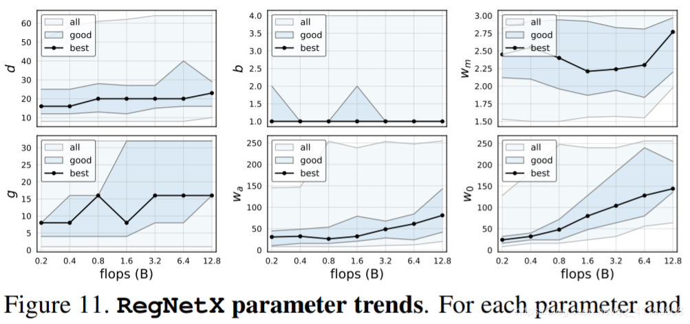
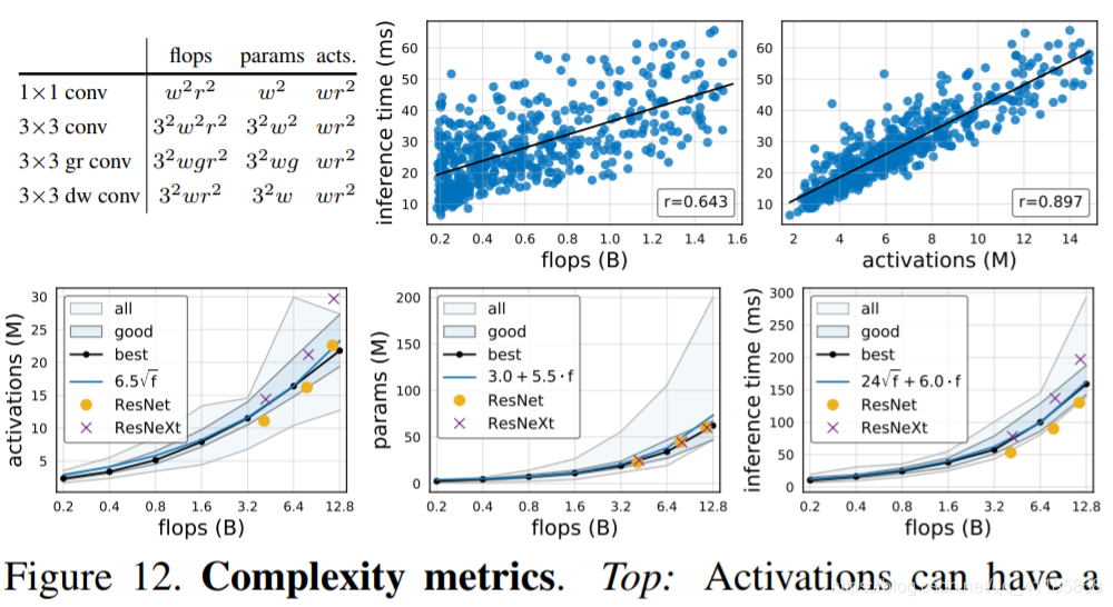
Figure 11. RegNetX parameter trends. For each parameter and each flop regime we apply an empirical bootstrap to obtain the range that contains best models with 95% confidence (shown with blue shading) and the likely best model (black line), see also Figure 2. We observe that for best models the depths d are remarkably stable across flops regimes, and b = 1 and wm ≈ 2.5 are best. Block and groups widths (wa, w0, g) tend to increase with flops. Figure 12. Complexity metrics. Top: Activations can have a stronger correlation to runtime on hardware accelerators than flops (we measure inference time for 64 images on an NVIDIA V100 GPU). Bottom: Trend analysis of complexity vs. flops and best fit curves (shown in blue) of the trends for best models (black curves). Figure 13. We refine RegNetX using various constraints (see text). The constrained variant (C) is best across all flop regimes while being more efficient in terms of parameters and activations. Figure 14. We evaluate RegNetX with alternate design choices. Left: Inverted bottleneck ( 1 8 ≤ b ≤ 1) degrades results and depthwise conv (g = 1) is even worse. Middle: Varying resolution r harms results. Right: RegNetY (Y=X+SE) improves the EDF. |
图11。RegNetX参数趋势。对于每个参数和每个触发器,我们应用经验自举法获得包含95%置信度的最佳模型(用蓝色底纹表示)和可能的最佳模型(黑线表示)的范围,参见图2。我们观察到,对于最佳模型,深度d在flops范围内非常稳定,b = 1和wm≈2.5是最佳的。块和组的宽度(wa、w0、g)随着拖放而增加。
图12。复杂性度量。Top:与flops相比,激活在硬件加速器上与运行时的相关性更强(我们在NVIDIA V100 GPU上测量64张图像的推断时间)。底部:趋势分析的复杂性与失败和最佳拟合曲线(蓝色显示)的趋势的最佳模型(黑色曲线)。
图13。我们使用各种约束来细化RegNetX(参见文本)。约束变式(C)在所有的触发器中都是最好的,同时在参数和激活方面更有效。 图14。我们评估RegNetX的备选设计选择。左:倒瓶颈(1 8≤b≤1)降低结果,深度conv (g = 1)更差。中间:变化的分辨率对结果有害。右:RegNetY (Y=X+SE)改善EDF。 |
4. Analyzing the RegNetX Design Space 分析RegNetX设计空间
We next further analyze the RegNetX design space and revisit common deep network design choices. Our analysis yields surprising insights that don’t match popular practice, which allows us to achieve good results with simple models. As the RegNetX design space has a high concentration of good models, for the following results we switch to sampling fewer models (100) but training them for longer (25 epochs) with a learning rate of 0.1 (see appendix). We do so to observe more fine-grained trends in network behavior. RegNet trends. We show trends in the RegNetX parameters across flop regimes in Figure 11. Remarkably, the depth of best models is stable across regimes (top-left), with an optimal depth of ∼20 blocks (60 layers). This is in contrast to the common practice of using deeper models for higher flop regimes. We also observe that the best models use a bottleneck ratio b of 1.0 (top-middle), which effectively removes the bottleneck (commonly used in practice). Next, we observe that the width multiplier wm of good models is ∼2.5 (top-right), similar but not identical to the popular recipe of doubling widths across stages. The remaining parameters (g, wa, w0) increase with complexity (bottom). |
接下来,我们将进一步分析RegNetX设计空间,并回顾常见的深度网络设计选择。我们的分析产生了与流行实践不匹配的惊人见解,这使我们能够用简单的模型获得良好的结果。 由于RegNetX设计空间拥有高度集中的优秀模型,对于以下结果,我们将转换为抽样较少的模型(100个),但对它们进行更长时间的培训(25个epoch),学习率为0.1(参见附录)。我们这样做是为了观察网络行为中更细微的趋势。 RegNet趋势。我们在图11中展示了在整个触发器中RegNetX参数的变化趋势。值得注意的是,最佳模型的深度在不同区域(左上)是稳定的,最优深度为∼20块(60层)。这与在更高的翻背越高的体制中使用更深的模式的惯例形成了对比。我们还观察到,最佳模型使用的瓶颈比b为1.0(上-中),这有效地消除了瓶颈(在实践中经常使用)。接下来,我们观察到好模型的宽度倍增器wm为∼2.5(右上角),这与流行的跨阶段加倍宽度的方法相似,但并不完全相同。其余参数(g、wa、w0)随复杂度增加而增加(底部)。 |
Complexity analysis. In addition to flops and parameters, we analyze network activations, which we define as the size of the output tensors of all conv layers (we list complexity measures of common conv operators in Figure 12, top-left). While not a common measure of network complexity, activations can heavily affect runtime on memory-bound hardware accelerators (e.g., GPUs, TPUs), for example, see Figure 12 (top). In Figure 12 (bottom), we observe that for the best models in the population, activations increase with the square-root of flops, parameters increase linearly, and runtime is best modeled using both a linear and a square-root term due to its dependence on both flops and activations. RegNetX constrained. Using these findings, we refine the RegNetX design space. First, based on Figure 11 (top), we set b = 1, d ≤ 40, and wm ≥ 2. Second, we limit parameters and activations, following Figure 12 (bottom). This yields fast, low-parameter, low-memory models without affecting accuracy. In Figure 13, we test RegNetX with theses constraints and observe that the constrained version is superior across all flop regimes. We use this version in §5, and further limit depth to 12 ≤ d ≤ 28 (see also Appendix D). |
复杂性分析。除了flops和参数之外,我们还分析了网络激活,我们将其定义为所有conv层的输出张量的大小(我们在图12(左上角)中列出了常见conv操作符的复杂性度量)。虽然激活不是测量网络复杂性的常用方法,但它会严重影响内存限制硬件加速器(例如,gpu、TPUs)上的运行时,参见图12(顶部)。在图12(底部)中,我们观察到,对于总体中的最佳模型,激活随flops的平方根增加而增加,参数线性增加,由于运行时对flops和激活的依赖性,最好同时使用线性和平方根项进行建模。 RegNetX受限。利用这些发现,我们改进了RegNetX设计空间。首先,根据图11 (top),我们令b = 1, d≤40,wm≥2。其次,我们限制参数和激活,如下图12(底部)所示。这将生成快速、低参数、低内存的模型,而不会影响准确性。在图13中,我们使用这些约束对RegNetX进行了测试,并观察到约束的版本在所有的触发器状态下都是优越的。我们在§5中使用这个版本,并进一步将深度限制为12≤d≤28(参见附录d)。 |
Alternate design choices. Modern mobile networks often employ the inverted bottleneck (b < 1) proposed in [25] along with depthwise conv [1] (g = 1). In Figure 14 (left), we observe that the inverted bottleneck degrades the EDF slightly and depthwise conv performs even worse relative to b = 1 and g ≥ 1 (see appendix for further analysis). Next, motivated by [29] who found that scaling the input image resolution can be helpful, we test varying resolution in Figure 14 (middle). Contrary to [29], we find that for RegNetX a fixed resolution of 224×224 is best, even at higher flops. SE. Finally, we evaluate RegNetX with the popular Squeeze-and-Excitation (SE) op [10] (we abbreviate X+SE as Y and refer to the resulting design space as RegNetY). In Figure 14 (right), we see that RegNetY yields good gains. |
替代设计选择。现代移动网络通常采用倒置瓶颈(b < 1)提出了[25]随着切除conv [1] (g = 1)。在图14(左),我们观察到倒置瓶颈略有降低了EDF,切除conv执行更糟糕的是相对于b = 1, g≥1进一步分析(见附录)。接下来,在[29]的启发下,我们测试了图14(中间)中变化的分辨率,[29]发现缩放输入图像分辨率是有帮助的。与[29]相反,我们发现对于RegNetX,固定的224×224分辨率是最好的,即使在更高的flops。 最后,我们使用流行的挤压-激励(SE) op[10]来评估RegNetX(我们将X+SE缩写为Y,并将最终的设计空间称为RegNetY)。在图14(右)中,我们看到RegNetY产生了良好的收益。 |
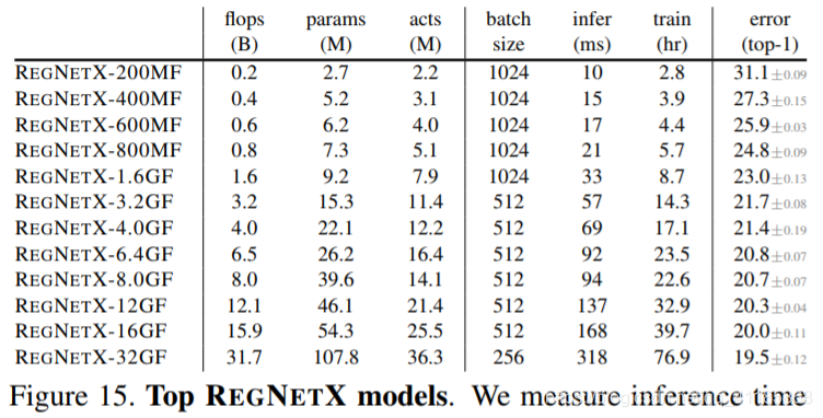
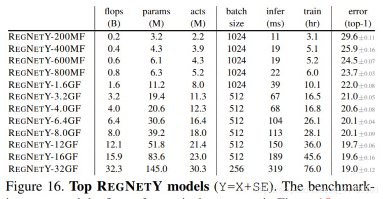
Figure 15. Top REGNETX models. We measure inference time for 64 images on an NVIDIA V100 GPU; train time is for 100 epochs on 8 GPUs with the batch size listed. Network diagram legends contain all information required to implement the models. Figure 16. Top REGNETY models (Y=X+SE). The benchmarking setup and the figure format is the same as in Figure 15. |
图15。顶级REGNETX模型。我们在NVIDIA V100 GPU上测量64幅图像的推理时间;在8个gpu上的训练时间为100个epoch,列出了批量大小。网络图图例包含实现模型所需的所有信息。 图16。顶级权威模型(Y=X+SE)。基准测试的设置和图的格式与图15相同。 |
5. Comparison to Existing Networks 与现有网络的比较
We now compare top models from the RegNetX and RegNetY design spaces at various complexities to the stateof-the-art on ImageNet [3]. We denote individual models using small caps, e.g. REGNETX. We also suffix the models with the flop regime, e.g. 400MF. For each flop regime, we pick the best model from 25 random settings of the RegNet parameters (d, g, wm, wa, w0), and re-train the top model 5 times at 100 epochs to obtain robust error estimates. Resulting top REGNETX and REGNETY models for each flop regime are shown in Figures 15 and 16, respectively. In addition to the simple linear structure and the trends we analyzed in §4, we observe an interesting pattern. Namely, the higher flop models have a large number of blocks in the third stage and a small number of blocks in the last stage. This is similar to the design of standard RESNET models. Moreover, we observe that the group width g increases with complexity, but depth d saturates for large models. |
我们现在比较的顶级模型从RegNetX和RegNetY设计空间在各种复杂的状态,对ImageNet[3]的艺术状态。我们使用小的大写字母来表示单个的模型,例如REGNETX。我们还在模型后面加上了触发器机制,例如400MF。对于每个触发器机制,我们从RegNet参数的25个随机设置(d、g、wm、wa、w0)中选出最佳模型,并在100个epoch时对top模型进行5次再训练,以获得可靠的误差估计。 图15和图16分别显示了每种翻牌制度的最高REGNETX和REGNETY模型。除了§4中分析的简单线性结构和趋势外,我们还观察到一个有趣的模式。即高阶触发器模型在第三阶段积木数量较多,在最后阶段积木数量较少。这与标准RESNET模型的设计类似。此外,我们观察到群宽度g随着复杂度的增加而增加,但是深度d对于大型模型来说是饱和的。 |
| Our goal is to perform fair comparisons and provide simple and easy-to-reproduce baselines. We note that along with better architectures, much of the recently reported gains in network performance are based on enhancements to the training setup and regularization scheme (see Table 7). As our focus is on evaluating network architectures, we perform carefully controlled experiments under the same training setup. In particular, to provide fair comparisons to classic work, we do not use any training-time enhancements. | 我们的目标是执行公平的比较,并提供简单且易于复制的基线。我们注意,以及更好的架构,最近的报道在网络性能是基于增强培训设置和正规化方案(见表7)。我们的重点是评估网络架构,我们表现的小心控制的实验设置在同样的培训。特别是,为了与经典作品进行公平的比较,我们没有使用任何培训时间的增强。 |
5.1. State-of-the-Art Comparison: Mobile Regime 最先进的比较:移动系统
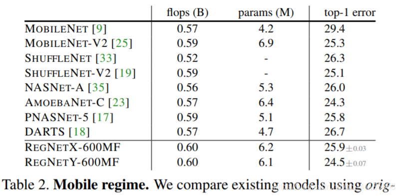
Much of the recent work on network design has focused on the mobile regime (∼600MF). In Table 2, we compare REGNET models at 600MF to existing mobile networks. We observe that REGNETS are surprisingly effective in this regime considering the substantial body of work on finding better mobile networks via both manual design [9, 25, 19] and NAS [35, 23, 17, 18]. We emphasize that REGNET models use our basic 100 epoch schedule with no regularization except weight decay, while most mobile networks use longer schedules with various enhancements, such as deep supervision [16], Cutout [4], DropPath [14], AutoAugment [2], and so on. As such, we hope our strong results obtained with a short training schedule without enhancements can serve as a simple baseline for future work. |
最近关于网络设计的大部分工作都集中在移动系统(∼600MF)上。在表2中,我们将600MF的REGNET模型与现有的移动网络进行了比较。我们注意到,考虑到通过手工设计[9,25,19]和NAS[35,23,17,18]来寻找更好的移动网络的大量工作,REGNETS在这种机制下的有效性令人惊讶。 我们强调,REGNET模型使用基本的100 epoch调度,除了权值衰减外没有任何正则化,而大多数移动网络使用更长的调度,并进行了各种增强,如深度监控[16]、删除[4]、删除路径[14]、自动增强[2]等等。因此,我们希望我们在短时间的培训计划中取得的良好结果可以作为未来工作的简单基线。 |
Table 2. Mobile regime. We compare existing models using originally reported errors to RegNet models trained in a basic setup. Our simple RegNet models achieve surprisingly good results given the effort focused on this regime in the past few years. Table 3. RESNE(X)T comparisons. (a) Grouped by activations, REGNETX show considerable gains (note that for each group GPU inference and training times are similar). (b) REGNETX models outperform RESNE(X)T models under fixed flops as well. Table 4. EFFICIENTNET comparisons using our standard training schedule. Under comparable training settings, REGNETY outperforms EFFICIENTNET for most flop regimes. Moreover, REGNET models are considerably faster, e.g., REGNETX-F8000 is about 5× faster than EFFICIENTNET-B5. Note that originally reported errors for EFFICIENTNET (shown grayed out), are much lower but use longer and enhanced training schedules, see Table 7. Figure 17. ResNe(X)t comparisons. REGNETX models versus RESNE(X)T-(50,101,152) under various complexity metrics. As all models use the identical components and training settings, all observed gains are from the design of the RegNetX design space Figure 18. EFFICIENTNET comparisons. REGNETs outperform the state of the art, especially when considering activations |
表2。移动的政权。我们将使用原始报告错误的现有模型与在基本设置中训练的RegNet模型进行比较。我们简单的RegNet模型取得了令人惊讶的好结果,因为在过去几年中我们一直致力于此机制。
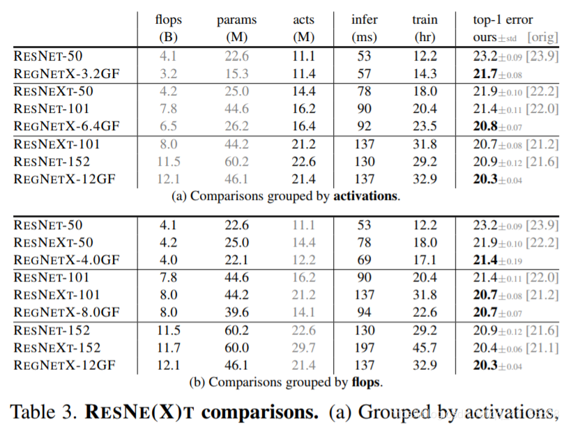
表3。RESNE T (X)的比较。(a)按照激活分组,REGNETX显示了相当大的增益(注意,对于每个组,GPU推断和训练时间是相似的)。(b) REGNETX模型的表现也优于RESNE(X)T模型。
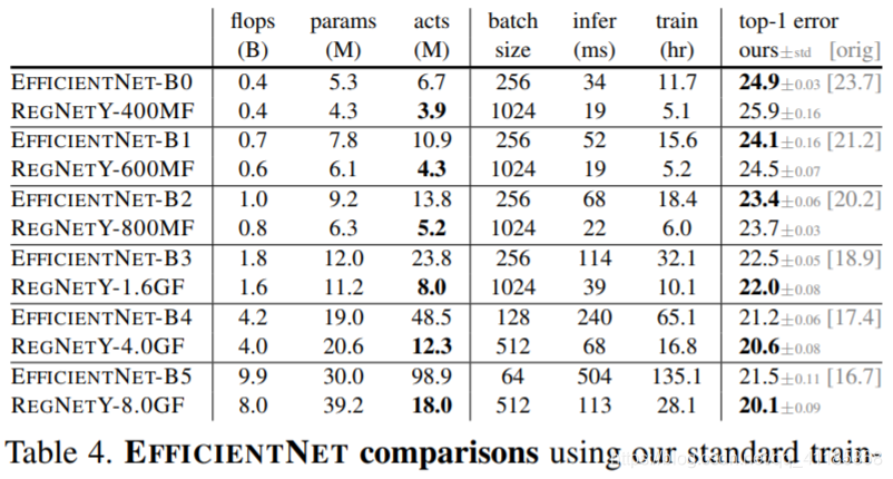
表4。使用我们的标准训练时间表进行有效的比较。在可比的训练环境下,REGNETY在大多数翻背战术中都表现得比有效网更好。此外,REGNET模型要快得多,例如,REGNET - f8000大约比efficient entnet - b5快5倍。请注意,efficient entnet最初报告的错误(显示为灰色)要低得多,但是使用更长的和增强的训练计划,见表7。
图17。ResNe t (X)的比较。在各种复杂度指标下,REGNETX模型与RESNE(X)T-(50,101,152)模型的比较。由于所有的模型都使用相同的组件和训练设置,所有观察到的收益都来自RegNetX设计空间的设计
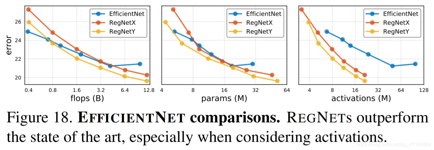
图18。EFFICIENTNET比较。regnet的性能优于当前的技术,特别是在考虑激活时 |
5.2. Standard Baselines Comparison: ResNe(X)t 标准基线比较:ResNe(X)t
Next, we compare REGNETX to standard RESNET [8] and RESNEXT [31] models. All of the models in this experiment come from the exact same design space, the former being manually designed, the latter being obtained through design space design. For fair comparisons, we compare REGNET and RESNE(X)T models under the same training setup (our standard REGNET training setup). We note that this results in improved RESNE(X)T baselines and highlights the importance of carefully controlling the training setup. Comparisons are shown in Figure 17 and Table 3. Overall, we see that REGNETX models, by optimizing the network structure alone, provide considerable improvements under all complexity metrics. We emphasize that good REGNET models are available across a wide range of compute regimes, including in low-compute regimes where good RESNE(X)T models are not available. |
接下来,我们将REGNETX与标准的RESNET[8]和RESNEXT[31]模型进行比较。本实验中所有的模型都来自于完全相同的设计空间,前者是人工设计,后者是通过设计空间设计得到的。为了进行公平的比较,我们在相同的训练设置(我们的标准REGNET训练设置)下比较REGNET和RESNE(X)T模型。我们注意到这导致了改进的RESNE(X)T基线,并强调了仔细控制培训设置的重要性。 比较结果如图17和表3所示。总的来说,我们看到,通过优化网络结构,REGNETX模型在所有复杂度指标下都提供了相当大的改进。我们强调,良好的REGNET模型适用于广泛的计算环境,包括在低计算环境中,因为没有良好的RESNE(X)T模型可用。 |
Table 3a shows comparisons grouped by activations (which can strongly influence runtime on accelerators such as GPUs). This setting is of particular interest to the research community where model training time is a bottleneck and will likely have more real-world use cases in the future, especially as accelerators gain more use at inference time (e.g., in self-driving cars). REGNETX models are quite effective given a fixed inference or training time budget. |
表3a显示了按激活分组的比较(这对加速程序(如gpu)的运行时有很大影响)。这个设置对研究社区特别有意义,因为模型训练时间是一个瓶颈,未来可能会有更多的真实世界用例,特别是在推断时间(例如,在自动驾驶汽车中)加速器获得更多的使用。给定一个固定的推论或训练时间预算,REGNETX模型是相当有效的。 |
5.3. State-of-the-Art Comparison: Full Regime 最先进的比较:完全制度
| We focus our comparison on EFFICIENTNET [29], which is representative of the state of the art and has reported impressive gains using a combination of NAS and an interesting model scaling rule across complexity regimes. To enable direct comparisons, and to isolate gains due to improvements solely of the network architecture, we opt to reproduce the exact EFFICIENTNET models but using our standard training setup, with a 100 epoch schedule and no regularization except weight decay (effect of longer schedule and stronger regularization are shown in Table 7). We optimize only lr and wd, see Figure 22 in appendix. This is the same setup as REGNET and enables fair comparisons. Results are shown in Figure 18 and Table 4. At low flops, EFFICIENTNET outperforms the REGNETY. At intermediate flops, REGNETY outperforms EFFICIENTNET, and at higher flops both REGNETX and REGNETY perform better. We also observe that for EFFICIENTNET, activations scale linearly with flops (due to the scaling of both resolution and depth), compared to activations scaling with the square-root of flops for REGNETs. This leads to slow GPU training and inference times for EFFICIENTNET. E.g., REGNETX-8000 is 5× faster than EFFICIENTNET-B5, while having lower error. | 我们将比较的重点放在了effecentnet[29]上,它代表了当前的技术水平,并报告了使用NAS和有趣的跨复杂性区域的模型缩放规则的组合所取得的令人印象深刻的成果。使直接比较,隔离收益仅仅由于改进的网络体系结构,我们选择复制的确切EFFICIENTNET模型但使用我们的标准培训设置,100时代的时间表,也没有正规化除了体重衰变(长时间表和更强的正规化的影响如表7所示),我们只优化lr和wd,参见图22在附录。这与REGNET的设置相同,支持公平的比较。结果如图18和表4所示。在性能较差时,efficient entnet的性能优于REGNETY。在中间的flops, REGNETY的表现优于efficiency entnet,在更高的flops, REGNETX和REGNETY的表现都更好。我们还观察到,对于effecentnet,激活与flops成线性关系(由于分辨率和深度的缩放),而对于REGNETs,激活与flops平方根成线性关系。这就导致了efficient entnet的GPU训练和推断速度变慢。例如,REGNETX-8000比efficient entnet - b5快5倍,同时具有更低的误差。 |
6. Conclusion 结论
| In this work, we present a new network design paradigm. Our results suggest that designing network design spaces is a promising avenue for future research. | 在这项工作中,我们提出了一个新的网络设计范例。研究结果表明,网络设计空间的设计是未来研究的重要方向。 |
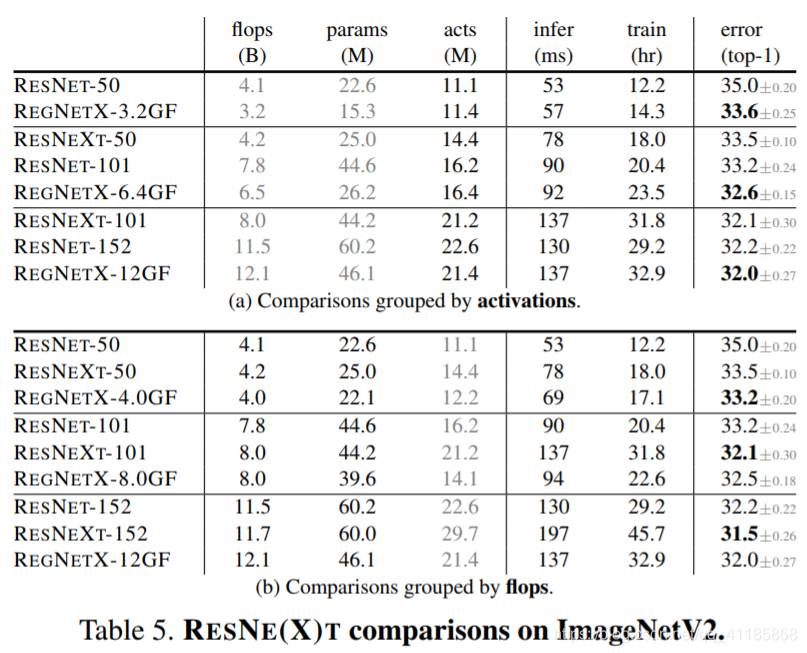
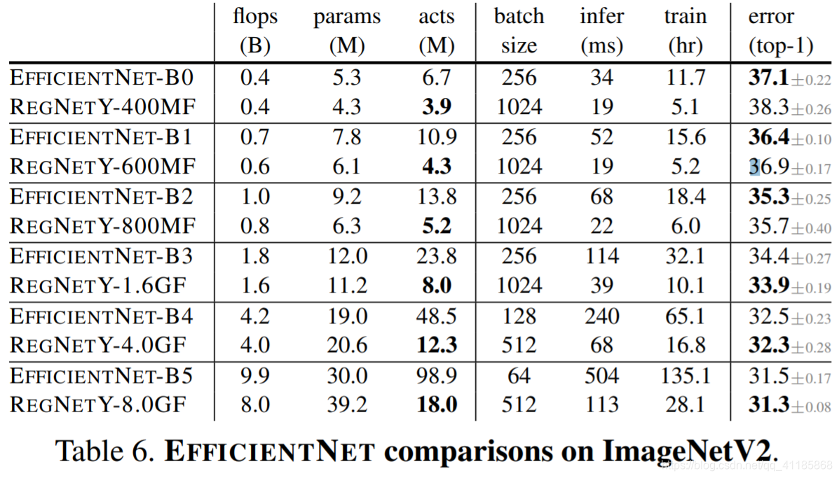
Table 5. RESNE(X)T comparisons on ImageNetV2 Table 6. EFFICIENTNET comparisons on ImageNetV2. |
表5所示。RESNE(X)T在ImageNetV2上的比较
表6所示。在ImageNetV2上的有效比较。
|
Figure 19. Additional ablations. Left: Fixed depth networks (d = 20) are effective across flop regimes. Middle: Three stage networks perform poorly at high flops. Right: Inverted bottleneck (b < 1) is also ineffective at high flops. See text for more context. Figure 20. Swish vs. ReLU. Left: RegNetY performs better with Swish than ReLU at 400MF but worse at 6.4GF. Middle: Results across wider flop regimes show similar trends. Right: If, however, g is restricted to be 1 (depthwise conv), Swish is much better. |
图19所示。额外的消融。左:固定深度网络(d = 20)在越空越有效。中间:三个阶段的网络在高失败时表现很差。右:反向瓶颈(b < 1)在高次失败时也是无效的。参见文本了解更多上下文。
图20。漂亮与ReLU。左图:RegNetY在400MF时的Swish表现比ReLU好,但在6.4GF时表现更差。中:更广泛的翻牌方法的结果显示了类似的趋势。正确:然而,如果g被限制为1(深度conv), Swish更好。 |

