官方参数解释:
Convolution 2D
tflearn.layers.conv.conv_2d (incoming, nb_filter, filter_size, strides=1, padding='same', activation='linear', bias=True, weights_init='uniform_scaling', bias_init='zeros', regularizer=None, weight_decay=0.001, trainable=True, restore=True, reuse=False, scope=None, name='Conv2D')
Input
4-D Tensor [batch, height, width, in_channels].
Output
4-D Tensor [batch, new height, new width, nb_filter].
Arguments
- incoming:
Tensor. Incoming 4-D Tensor. - nb_filter:
int. The number of convolutional filters. - filter_size:
intorlist of int. Size of filters. - strides: 'int
or list ofint`. Strides of conv operation. Default: [1 1 1 1]. - padding:
strfrom"same", "valid". Padding algo to use. Default: 'same'. - activation:
str(name) orfunction(returning aTensor) or None. Activation applied to this layer (see tflearn.activations). Default: 'linear'. - bias:
bool. If True, a bias is used. - weights_init:
str(name) orTensor. Weights initialization. (see tflearn.initializations) Default: 'truncated_normal'. - bias_init:
str(name) orTensor. Bias initialization. (see tflearn.initializations) Default: 'zeros'. - regularizer:
str(name) orTensor. Add a regularizer to this layer weights (see tflearn.regularizers). Default: None. - weight_decay:
float. Regularizer decay parameter. Default: 0.001. - trainable:
bool. If True, weights will be trainable. - restore:
bool. If True, this layer weights will be restored when loading a model. - reuse:
bool. If True and 'scope' is provided, this layer variables will be reused (shared). - scope:
str. Define this layer scope (optional). A scope can be used to share variables between layers. Note that scope will override name. - name: A name for this layer (optional). Default: 'Conv2D'.
代码:
# 64 filters
net
=
tflearn.conv_2d(net,
64
,
3
, activation
=
'relu'
)

其中的filter(卷积核)就是
[1 0 1
0 1 0
1 0 1],size=3
因为设置了64个filter,那么卷积操作后有64个卷积结果作为输入的特征(feature map)。难道后面激活函数就是因为选择部分激活???


图的原文:http://cs231n.github.io/convolutional-networks/
如果一个卷积层有4个feature map,那是不是就有4个卷积核?
是的。
这4个卷积核如何定义?

通常是随机初始化再用BP算梯度做训练。如果数据少或者没有labeled data的话也可以考虑用K-means的K个中心点,逐层做初始化。

卷积核是学习的。卷积核是因为权重的作用方式跟卷积一样,所以叫卷积层,其实你还是可以把它看成是一个parameter layer,需要更新的。
--------------------------------------------------------------------------------------------------

下面内容摘自:http://blog.csdn.net/bugcreater/article/details/53293075
- from __future__ import division, print_function, absolute_import
- import tflearn
- from tflearn.layers.core import input_data, dropout, fully_connected
- from tflearn.layers.conv import conv_2d, max_pool_2d
- from tflearn.layers.normalization import local_response_normalization
- from tflearn.layers.estimator import regression
- #加载大名顶顶的mnist数据集(http://yann.lecun.com/exdb/mnist/)
- import tflearn.datasets.mnist as mnist
- X, Y, testX, testY = mnist.load_data(one_hot=True)
- X = X.reshape([-1, 28, 28, 1])
- testX = testX.reshape([-1, 28, 28, 1])
- network = input_data(shape=[None, 28, 28, 1], name='input')
- # CNN中的卷积操作,下面会有详细解释
- network = conv_2d(network, 32, 3, activation='relu', regularizer="L2")
- # 最大池化操作
- network = max_pool_2d(network, 2)
- # 局部响应归一化操作
- network = local_response_normalization(network)
- network = conv_2d(network, 64, 3, activation='relu', regularizer="L2")
- network = max_pool_2d(network, 2)
- network = local_response_normalization(network)
- # 全连接操作
- network = fully_connected(network, 128, activation='tanh')
- # dropout操作
- network = dropout(network, 0.8)
- network = fully_connected(network, 256, activation='tanh')
- network = dropout(network, 0.8)
- network = fully_connected(network, 10, activation='softmax')
- # 回归操作
- network = regression(network, optimizer='adam', learning_rate=0.01,
- loss='categorical_crossentropy', name='target')
- # Training
- # DNN操作,构建深度神经网络
- model = tflearn.DNN(network, tensorboard_verbose=0)
- model.fit({'input': X}, {'target': Y}, n_epoch=20,
- validation_set=({'input': testX}, {'target': testY}),
- snapshot_step=100, show_metric=True, run_id='convnet_mnist')
关于conv_2d函数,在源码里是可以看到总共有14个参数,分别如下:
1.incoming: 输入的张量,形式是[batch, height, width, in_channels]
2.nb_filter: filter的个数
3.filter_size: filter的尺寸,是int类型
4.strides: 卷积操作的步长,默认是[1,1,1,1]
5.padding: padding操作时标志位,"same"或者"valid",默认是“same”
6.activation: 激活函数(ps:这里需要了解的知识很多,会单独讲)
7.bias: bool量,如果True,就是使用bias
8.weights_init: 权重的初始化
9.bias_init: bias的初始化,默认是0,比如众所周知的线性函数y=wx+b,其中的w就相当于weights,b就是bias
10.regularizer: 正则项(这里需要讲解的东西非常多,会单独讲)
11.weight_decay: 权重下降的学习率
12.trainable: bool量,是否可以被训练
13.restore: bool量,训练的模型是否被保存
14.name: 卷积层的名称,默认是"Conv2D"
关于max_pool_2d函数,在源码里有5个参数,分别如下:
1.incoming ,类似于conv_2d里的incoming
2.kernel_size:池化时核的大小,相当于conv_2d时的filter的尺寸
3.strides:类似于conv_2d里的strides
4.padding:同上
5.name:同上
看了这么多参数,好像有些迷糊,我先用一张图解释下每个参数的意义。
其中的filter就是
[1 0 1
0 1 0
1 0 1],size=3,由于每次移动filter都是一个格子,所以strides=1.
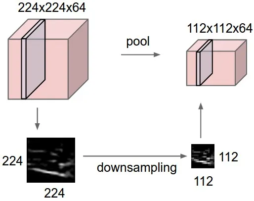
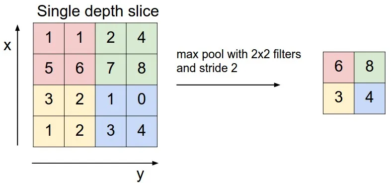
关于最大池化可以看看下面这张图,这里面 strides=1,kernel_size =2(就是每个颜色块的大小),图中示意的最大池化(可以提取出显著信息,比如在进行文本分析时可以提取一句话里的关键字,以及图像处理中显著颜色,纹理等),关于池化这里多说一句,有时需要平均池化,有时需要最小池化。
下面说说其中的padding操作,做图像处理的人对于这个操作应该不会陌生,说白了,就是填充。比如你对图像做卷积操作,比如你用的3×3的卷积核,在进行边上操作时,会发现卷积核已经超过原图像,这时需要把原图像进行扩大,扩大出来的就是填充,基本都填充0。
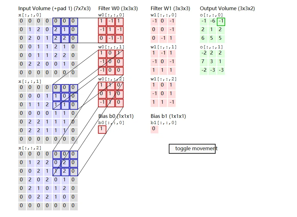
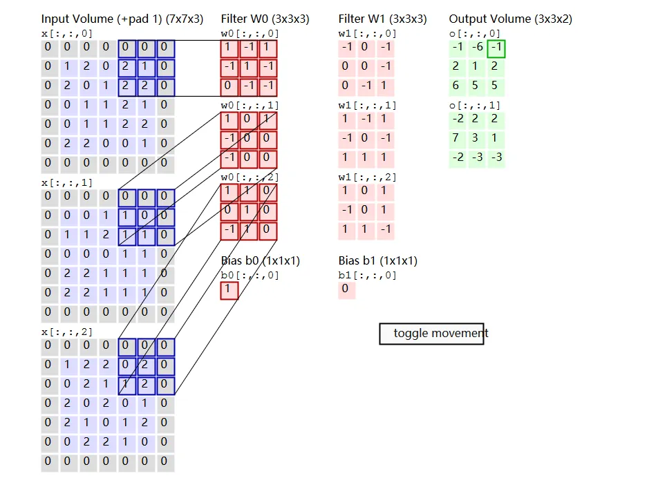
Convolution Demo. Below is a running demo of a CONV layer. Since 3D volumes are hard to visualize, all the volumes (the input volume (in blue), the weight volumes (in red), the output volume (in green)) are visualized with each depth slice stacked in rows. The input volume is of size W, and the CONV layer parameters are K. That is, we have two filters of size 3×3, and they are applied with a stride of 2. Therefore, the output volume size has spatial size (5 - 3 + 2)/2 + 1 = 3. Moreover, notice that a padding of P
General pooling. In addition to max pooling, the pooling units can also perform other functions, such as average pooling or even L2-norm pooling. Average pooling was often used historically but has recently fallen out of favor compared to the max pooling operation, which has been shown to work better in practice.
本文转自张昺华-sky博客园博客,原文链接:http://www.cnblogs.com/bonelee/p/7908217.html,如需转载请自行联系原作者