
💡💡💡本文内容:如何用自己的数据集训练YOLOv13,在NEU-DET任务中YOLOv13原始mAP50为0.742;yolov13-MSCA原始mAP50为0.742提升至0.746;yolov13-MSCA1原始mAP50为0.742提升至0.749;yolov13-MSCA2原始mAP50为0.742提升至0.749

博主简介
AI小怪兽,YOLO骨灰级玩家,1)YOLOv5、v7、v8、v9、v10、11、v12、v13优化创新,轻松涨点和模型轻量化;2)目标检测、语义分割、OCR、分类等技术孵化,赋能智能制造,工业项目落地经验丰富;

1.YOLOv13介绍

论文:[2506.17733] YOLOv13: Real-Time Object Detection with Hypergraph-Enhanced Adaptive Visual Perception
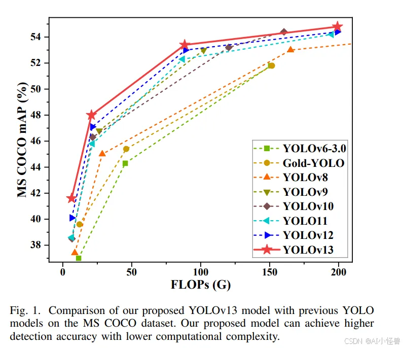
摘要—YOLO 系列模型因其卓越的准确性和计算效率在实时目标检测领域占据主导地位。然而,无论是 YOLO11 及更早版本的卷积架构,还是 YOLOv12 引入的基于区域的自注意力机制,都仅限于局部信息聚合和成对相关性建模,缺乏捕捉全局多对多高阶相关性的能力,这限制了在复杂场景下的检测性能。本文提出了一种准确且轻量化的 YOLOv13 目标检测器。为应对上述挑战,我们提出了一种基于超图的自适应相关性增强(HyperACE)机制,通过超图计算自适应地利用潜在的高阶相关性,克服了以往方法仅基于成对相关性建模的限制,实现了高效的全局跨位置和跨尺度特征融合与增强。随后,我们基于 HyperACE 提出了全链路聚合与分配(FullPAD)范式,通过将相关性增强特征分配到整个网络,有效实现了全网的细粒度信息流和表征协同。最后,我们提出用深度可分离卷积代替常规的大核卷积,并设计了一系列块结构,在不牺牲性能的前提下显著降低了参数量和计算复杂度。我们在广泛使用的 MS COCO 基准测试上进行了大量实验,结果表明,我们的方法在参数更少、浮点运算量更少的情况下达到了最先进性能。具体而言,我们的 YOLOv13-N 相比 YOLO11-N 提升了 3.0% 的 mAP,相比 YOLOv12-N 提升了 1.5% 的 mAP。

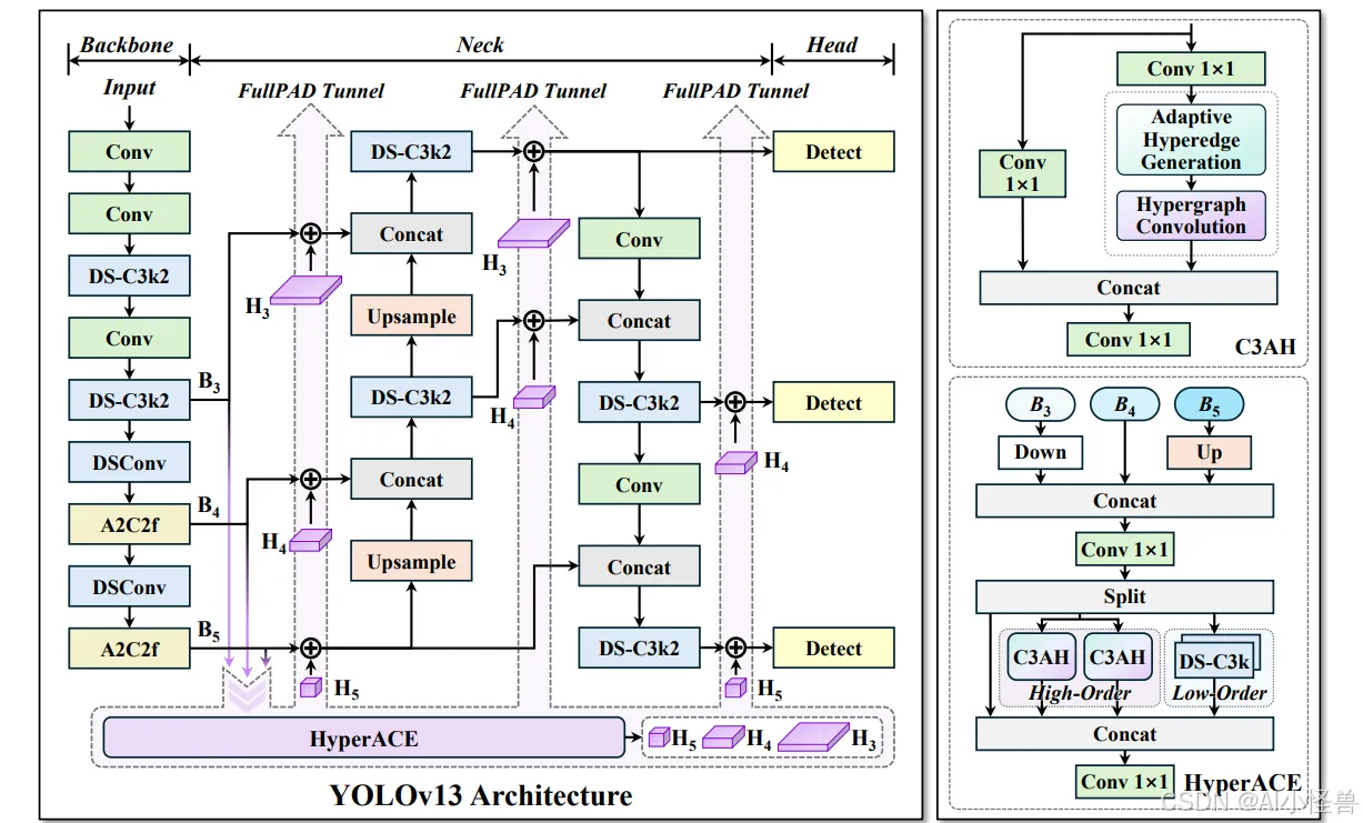
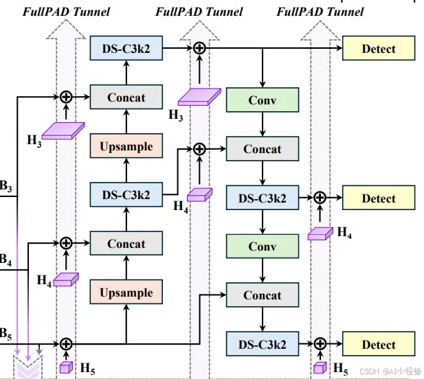
以往的 YOLO 系列遵循 “骨干网络 → 颈部网络 → 检测头” 的计算范式,这本质上限定了信息流的充分传输。相比之下,我们的模型通过超图自适应关联增强(HyperACE)机制,实现全链路特征聚合与分配(FullPAD),从而增强传统的 YOLO 架构。因此,我们提出的方法在整个网络中实现了细粒度的信息流和表征协同,能够改善梯度传播并显著提升检测性能。具体而言,如图 2 所示,我们的 YOLOv13 模型首先使用类似以往工作的骨干网络提取多尺度特征图 B1、B2、B3、B4、B5,但其中的大核卷积被我们提出的轻量化 DS-C3k2 模块取代。然后,与传统 YOLO 方法直接将 B3、B4 和 B5 输入颈部网络不同,我们的方法将这些特征收集并传递到提出的 HyperACE 模块中,实现跨尺度跨位置特征的高阶关联自适应建模和特征增强。随后,我们的 FullPAD 范式利用三个独立通道,将关联增强后的特征分别分配到骨干网络与颈部网络的连接处、颈部网络的内部层以及颈部网络与检测头的连接处,以优化信息流。最后,颈部网络的输出特征图被传递到检测头中,实现多尺度目标检测。

ultralytics/cfg/models/v13/yolov13.yaml
nc: 80 # number of classes
scales: # model compound scaling constants, i.e. 'model=yolov13n.yaml' will call yolov13.yaml with scale 'n'
  # [depth, width, max_channels]
  n: [0.50, 0.25, 1024]   # Nano
  s: [0.50, 0.50, 1024]   # Small
  l: [1.00, 1.00, 512]    # Large
  x: [1.00, 1.50, 512]    # Extra Large
backbone:
  # [from, repeats, module, args]
  - [-1, 1, Conv,  [64, 3, 2]] # 0-P1/2
  - [-1, 1, Conv,  [128, 3, 2, 1, 2]] # 1-P2/4
  - [-1, 2, DSC3k2,  [256, False, 0.25]]
  - [-1, 1, Conv,  [256, 3, 2, 1, 4]] # 3-P3/8
  - [-1, 2, DSC3k2,  [512, False, 0.25]]
  - [-1, 1, DSConv,  [512, 3, 2]] # 5-P4/16
  - [-1, 4, A2C2f, [512, True, 4]]
  - [-1, 1, DSConv,  [1024, 3, 2]] # 7-P5/32
  - [-1, 4, A2C2f, [1024, True, 1]] # 8
head:
  - [[4, 6, 8], 2, HyperACE, [512, 8, True, True, 0.5, 1, "both"]]
  - [-1, 1, nn.Upsample, [None, 2, "nearest"]]
  - [ 9, 1, DownsampleConv, []]
  - [[6, 9], 1, FullPAD_Tunnel, []]  #12
  - [[4, 10], 1, FullPAD_Tunnel, []]  #13
  - [[8, 11], 1, FullPAD_Tunnel, []] #14

  - [-1, 1, nn.Upsample, [None, 2, "nearest"]]
  - [[-1, 12], 1, Concat, [1]] # cat backbone P4
  - [-1, 2, DSC3k2, [512, True]] # 17
  - [[-1, 9], 1, FullPAD_Tunnel, []]  #18
  - [17, 1, nn.Upsample, [None, 2, "nearest"]]
  - [[-1, 13], 1, Concat, [1]] # cat backbone P3
  - [-1, 2, DSC3k2, [256, True]] # 21
  - [10, 1, Conv, [256, 1, 1]]
  - [[21, 22], 1, FullPAD_Tunnel, []]  #23

  - [-1, 1, Conv, [256, 3, 2]]
  - [[-1, 18], 1, Concat, [1]] # cat head P4
  - [-1, 2, DSC3k2, [512, True]] # 26
  - [[-1, 9], 1, FullPAD_Tunnel, []]
  - [26, 1, Conv, [512, 3, 2]]
  - [[-1, 14], 1, Concat, [1]] # cat head P5
  - [-1, 2, DSC3k2, [1024,True]] # 30 (P5/32-large)
  - [[-1, 11], 1, FullPAD_Tunnel, []]

  - [[23, 27, 31], 1, Detect, [nc]] # Detect(P3, P4, P5)

1.1 HyperACE
超图自适应相关性增强机制 HyperACE
- 超图理论借鉴与创新 :借鉴超图理论,将多尺度特征图的像素视为超图顶点,不同的是,传统超图方法依赖手工设定参数构建超边,而 HyperACE 设计了可学习的超边生成模块,能自适应地学习并构建超边,动态探索不同特征顶点间的潜在关联。
- 超图卷积操作 :在生成自适应超边后,通过超图卷积操作进行特征聚合与增强。每条超边先从其连接的所有顶点处聚合信息形成高阶特征,再将这些高阶特征传播回各个顶点,更新与增强顶点特征,从而实现高效地跨位置和跨尺度的特征融合与增强,强化不同尺度特征间的语义关联,对小目标和密集目标检测效果显著。
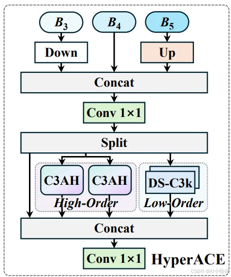

class HyperACE(nn.Module):
    """
    Hypergraph-based Adaptive Correlation Enhancement (HyperACE).
    This is the core module of YOLOv13, designed to model both global high-order correlations and
    local low-order correlations. It first fuses multi-scale features, then processes them through parallel
    branches: two C3AH branches for high-order modeling and a lightweight DSConv-based branch for
    low-order feature extraction.
    Attributes:
        c1 (int): Number of input channels for the fuse module.
        c2 (int): Number of output channels for the entire block.
        n (int, optional): Number of blocks in the low-order branch. Defaults to 1.
        num_hyperedges (int, optional): Number of hyperedges for the C3AH branches. Defaults to 8.
        dsc3k (bool, optional): If True, use DSC3k in the low-order branch; otherwise, use DSBottleneck. Defaults to True.
        shortcut (bool, optional): Whether to use shortcuts in the low-order branch. Defaults to False.
        e1 (float, optional): Expansion ratio for the main hidden channels. Defaults to 0.5.
        e2 (float, optional): Expansion ratio within the C3AH branches. Defaults to 1.
        context (str, optional): Context type for C3AH branches. Defaults to "both".
        channel_adjust (bool, optional): Passed to FuseModule for channel configuration. Defaults to True.
    Methods:
        forward: Performs a forward pass through the HyperACE module.
    Examples:
        >>> import torch
        >>> model = HyperACE(c1=64, c2=256, n=1, num_hyperedges=8)
        >>> x_list = [torch.randn(2, 64, 64, 64), torch.randn(2, 64, 32, 32), torch.randn(2, 64, 16, 16)]
        >>> output = model(x_list)
        >>> print(output.shape)
        torch.Size([2, 256, 32, 32])
    """
    def __init__(self, c1, c2, n=1, num_hyperedges=8, dsc3k=True, shortcut=False, e1=0.5, e2=1, context="both", channel_adjust=True):
        super().__init__()
        self.c = int(c2 * e1)
        self.cv1 = Conv(c1, 3 * self.c, 1, 1)
        self.cv2 = Conv((4 + n) * self.c, c2, 1)
        self.m = nn.ModuleList(
            DSC3k(self.c, self.c, 2, shortcut, k1=3, k2=7) if dsc3k else DSBottleneck(self.c, self.c, shortcut=shortcut) for _ in range(n)
        )
        self.fuse = FuseModule(c1, channel_adjust)
        self.branch1 = C3AH(self.c, self.c, e2, num_hyperedges, context)
        self.branch2 = C3AH(self.c, self.c, e2, num_hyperedges, context)

    def forward(self, X):
        x = self.fuse(X)
        y = list(self.cv1(x).chunk(3, 1))
        out1 = self.branch1(y[1])
        out2 = self.branch2(y[1])
        y.extend(m(y[-1]) for m in self.m)
        y[1] = out1
        y.append(out2)
        return self.cv2(torch.cat(y, 1))

代码位置ultralytics/nn/modules/block.py
1.2 FullPAD_Tunnel
全流程聚合 - 分发范式 FullPAD
- 多通道特征传递 :打破传统的 “骨干→颈部→头部” 单向计算范式,通过三条独立通路传递特征,即主干 - 颈部连接层、颈部内部层、颈部 - 头部连接层,将 HyperACE 聚合后的多尺度特征,通过这些 “隧道” 分发回网络的不同位置,实现细粒度信息流与全流程表征协同。
- 改善梯度传播 :该范式有效解决了梯度消失或爆炸问题,显着改善了梯度传播效率,从而提升模型整体的检测性能,使模型在复杂场景下能够更好地捕捉目标特征,提高检测的准确性和稳定性。

class FullPAD_Tunnel(nn.Module):
    """
    A gated fusion module for the Full-Pipeline Aggregation-and-Distribution (FullPAD) paradigm.
    This module implements a gated residual connection used to fuse features. It takes two inputs: the original
    feature map and a correlation-enhanced feature map. It then computes `output = original + gate * enhanced`,
    where `gate` is a learnable scalar parameter that adaptively balances the contribution of the enhanced features.
    Methods:
        forward: Performs the gated fusion of two input feature maps.
    Examples:
        >>> import torch
        >>> model = FullPAD_Tunnel()
        >>> original_feature = torch.randn(2, 64, 32, 32)
        >>> enhanced_feature = torch.randn(2, 64, 32, 32)
        >>> output = model([original_feature, enhanced_feature])
        >>> print(output.shape)
        torch.Size([2, 64, 32, 32])
    """
    def __init__(self):
        super().__init__()
        self.gate = nn.Parameter(torch.tensor(0.0))
    def forward(self, x):
        out = x[0] + self.gate * x[1]
        return out

代码位置ultralytics/nn/modules/block.py
1.3 DSC3k2
基于深度可分离卷积的轻量化模块
- 模块创新与替代 :采用深度可分离卷积构建了 DSConv、DS-Bottleneck、DS-C3k 等模块,替代传统的大核卷积。例如使用 DS-C3k2 模块作为轻量化的骨干网络提取多尺度特征,在保持感受野的同时,大幅降低了参数量与计算量,提高了模型的计算效率。
- 性能与效率平衡 :在几乎不牺牲性能的前提下,显著减少了模型的参数量和计算复杂度,使得 YOLOv13 能够在保持较高检测精度的同时,具备更快的推理速度,适合实时目标检测应用场景,降低了模型的部署难度和资源消耗。
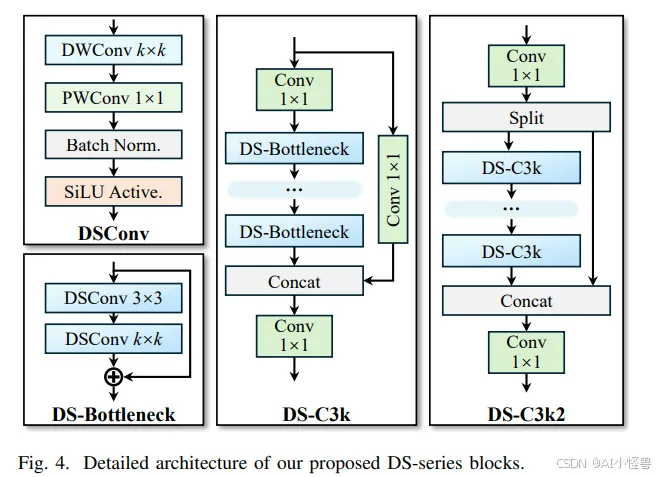

class DSC3k2(C2f):
    """
    An improved C3k2 module that uses lightweight depthwise separable convolution blocks.
    This class redesigns C3k2 module, replacing its internal processing blocks with either DSBottleneck
    or DSC3k modules.
    Attributes:
        c1 (int): Number of input channels.
        c2 (int): Number of output channels.
        n (int, optional): Number of internal processing blocks to stack. Defaults to 1.
        dsc3k (bool, optional): If True, use DSC3k as the internal block. If False, use DSBottleneck. Defaults to False.
        e (float, optional): Expansion ratio for the C2f module's hidden channels. Defaults to 0.5.
        g (int, optional): Number of groups for grouped convolution (passed to parent C2f). Defaults to 1.
        shortcut (bool, optional): Whether to use shortcut connections in the internal blocks. Defaults to True.
        k1 (int, optional): Kernel size for the first DSConv in internal blocks. Defaults to 3.
        k2 (int, optional): Kernel size for the second DSConv in internal blocks. Defaults to 7.
        d2 (int, optional): Dilation for the second DSConv in internal blocks. Defaults to 1.
    Methods:
        forward: Performs a forward pass through the DSC3k2 module (inherited from C2f).
    Examples:
        >>> import torch
        >>> # Using DSBottleneck as internal block
        >>> model1 = DSC3k2(c1=64, c2=64, n=2, dsc3k=False)
        >>> x = torch.randn(2, 64, 128, 128)
        >>> output1 = model1(x)
        >>> print(f"With DSBottleneck: {output1.shape}")
        With DSBottleneck: torch.Size([2, 64, 128, 128])
        >>> # Using DSC3k as internal block
        >>> model2 = DSC3k2(c1=64, c2=64, n=1, dsc3k=True)
        >>> output2 = model2(x)
        >>> print(f"With DSC3k: {output2.shape}")
        With DSC3k: torch.Size([2, 64, 128, 128])
    """
    def __init__(
        self,
        c1,
        c2,
        n=1,
        dsc3k=False,
        e=0.5,
        g=1,
        shortcut=True,
        k1=3,
        k2=7,
        d2=1
    ):
        super().__init__(c1, c2, n, shortcut, g, e)
        if dsc3k:
            self.m = nn.ModuleList(
                DSC3k(
                    self.c, self.c,
                    n=2,
                    shortcut=shortcut,
                    g=g,
                    e=1.0,
                    k1=k1,
                    k2=k2,
                    d2=d2
                )
                for _ in range(n)
            )
        else:
            self.m = nn.ModuleList(
                DSBottleneck(
                    self.c, self.c,
                    shortcut=shortcut,
                    e=1.0,
                    k1=k1,
                    k2=k2,
                    d2=d2
                )
                for _ in range(n)
            )

代码位置ultralytics/nn/modules/block.py
2.NEU-DET数据集介绍
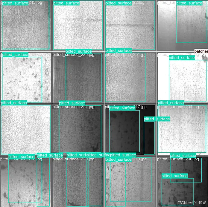
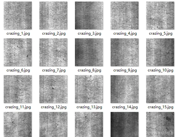
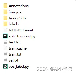
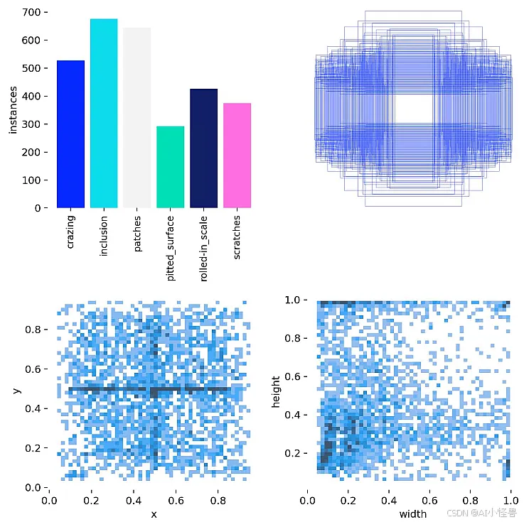
NEU-DET钢材表面缺陷共有六大类,一共1800张,
类别分别为:'crazing','inclusion','patches','pitted_surface','rolled-in_scale','scratches'

数据集下载地址:
https://download.csdn.net/download/m0_63774211/89846379?spm=1001.2014.3001.5503


标签可视化:

3.MSCAAttention注意力介绍

论文:https://arxiv.org/pdf/2209.08575.pdf
摘要:介绍了一种用于语义分割的简单卷积网络体系结构SegNeXt。由于在编码空间信息时自我注意的效率,最近基于Transformer的模型已主导语义分割领域。在本文中,我们证明了卷积注意比Transformer中的自注意机制更有效地编码上下文信息。本文对已有成功分割方案进行了重审视并发现了几个有助于性能提升的关键成分,进而促使我们设计了一种新型的卷积注意力架构方案SegNeXt。在没有任何花哨的成分下,我们的SegNeXt显着改善了以前在流行基准测试 (包括ADE20K,Cityscapes,COCO-Stuff,Pascal VOC,Pascal Context和iSAID) 上最先进的方法的性能。值得注意的是,SegNeXt的性能优于EfficientNet-L2 w/ NAS-FPN,并且仅使用其1/10参数在Pascal VOC 2012测试一下排行榜上实现90.6% mIoU。与ad20k数据集上具有相同或更少计算的最新方法相比,SegNeXt平均实现了约2.0% mIoU改进。
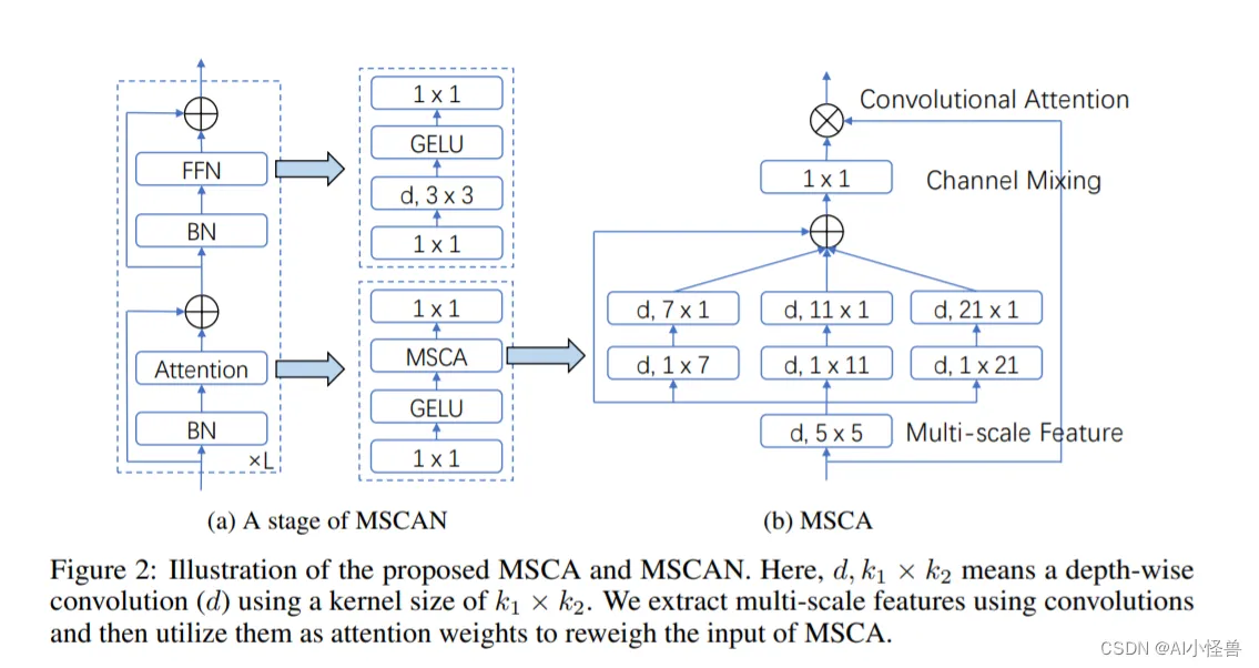
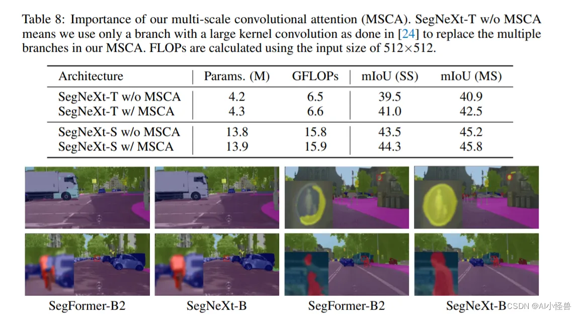
设计了一种新的多尺度卷积注意(MSCA)模块。如图2 (a)所示,MSCA包含三个部分:深度卷积聚合局部信息,多分支深度条卷积捕获多尺度上下文,以及1×1卷积建模不同通道之间的关系。


4.实验结果分析
4.1 原始结果
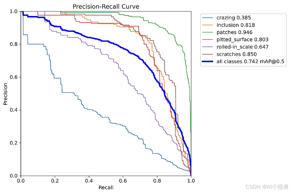
YOLOv13原始mAP50为0.742
YOLOv13n summary: 535 layers, 2,449,065 parameters, 0 gradients, 6.2 GFLOPs
                 Class     Images  Instances      Box(P          R      mAP50      mAP75  mAP50-95): 100%|██████████| 16/16 [00:11<00:00,  1.37it/s]
                   all        486       1069      0.749      0.659      0.742      0.433      0.426
               crazing         69        149      0.781      0.143      0.385     0.0432      0.128
             inclusion         87        222      0.773       0.77      0.818      0.425       0.45
               patches         92        243      0.824      0.905      0.946      0.752      0.614
        pitted_surface         93        130      0.779      0.746      0.803      0.581       0.54
       rolled-in_scale         81        171       0.71      0.544      0.647      0.219        0.3
             scratches         90        154      0.629      0.844       0.85       0.58      0.523


4.2 yaml修改
提供多种 MSCAAttention修改方式,分别加在网络不同位置,总有一种适合你的数据集
4.2.1 yolov13-MSCA.yaml
nc: 80 # number of classes
scales: # model compound scaling constants, i.e. 'model=yolov13n.yaml' will call yolov13.yaml with scale 'n'
  # [depth, width, max_channels]
  n: [0.50, 0.25, 1024]   # Nano
  s: [0.50, 0.50, 1024]   # Small
  l: [1.00, 1.00, 512]    # Large
  x: [1.00, 1.50, 512]    # Extra Large
backbone:
  # [from, repeats, module, args]
  - [-1, 1, Conv,  [64, 3, 2]] # 0-P1/2
  - [-1, 1, Conv,  [128, 3, 2, 1, 2]] # 1-P2/4
  - [-1, 2, DSC3k2,  [256, False, 0.25]]
  - [-1, 1, Conv,  [256, 3, 2, 1, 4]] # 3-P3/8
  - [-1, 2, DSC3k2,  [512, False, 0.25]]
  - [-1, 1, DSConv,  [512, 3, 2]] # 5-P4/16
  - [-1, 4, A2C2f, [512, True, 4]]
  - [-1, 1, DSConv,  [1024, 3, 2]] # 7-P5/32
  - [-1, 4, A2C2f, [1024, True, 1]] # 8
  - [-1, 1, MSCAAttention, []] # 9
head:
  - [[4, 6, 8], 2, HyperACE, [512, 8, True, True, 0.5, 1, "both"]]
  - [-1, 1, nn.Upsample, [None, 2, "nearest"]]
  - [ 10, 1, DownsampleConv, []]
  - [[6, 10], 1, FullPAD_Tunnel, []]  #13
  - [[4, 11], 1, FullPAD_Tunnel, []]  #14
  - [[9, 12], 1, FullPAD_Tunnel, []] #15

  - [-1, 1, nn.Upsample, [None, 2, "nearest"]]
  - [[-1, 13], 1, Concat, [1]] # cat backbone P4
  - [-1, 2, DSC3k2, [512, True]] # 18
  - [[-1, 10], 1, FullPAD_Tunnel, []]  #19
  - [18, 1, nn.Upsample, [None, 2, "nearest"]]
  - [[-1, 14], 1, Concat, [1]] # cat backbone P3
  - [-1, 2, DSC3k2, [256, True]] # 22
  - [11, 1, Conv, [256, 1, 1]]
  - [[22, 23], 1, FullPAD_Tunnel, []]  #24

  - [-1, 1, Conv, [256, 3, 2]]
  - [[-1, 19], 1, Concat, [1]] # cat head P4
  - [-1, 2, DSC3k2, [512, True]] # 27
  - [[-1, 10], 1, FullPAD_Tunnel, []]
  - [27, 1, Conv, [512, 3, 2]]
  - [[-1, 15], 1, Concat, [1]] # cat head P5
  - [-1, 2, DSC3k2, [1024,True]] # 31 (P5/32-large)
  - [[-1, 12], 1, FullPAD_Tunnel, []]

  - [[24, 28, 32], 1, Detect, [nc]] # Detect(P3, P4, P5)

原始mAP50为0.742提升至0.746
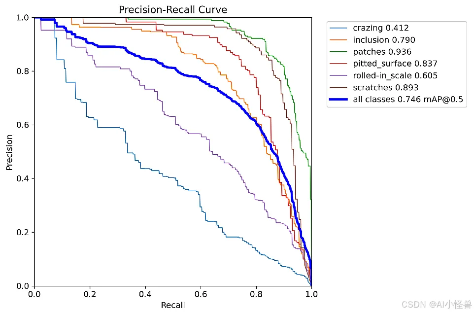

YOLOv13n-MSCA summary: 544 layers, 2,543,017 parameters, 0 gradients, 6.3 GFLOPs
                 Class     Images  Instances      Box(P          R      mAP50      mAP75  mAP50-95): 100%|██████████| 16/16 [00:18<00:00,  1.14s/it]
                   all        486       1069      0.668      0.699      0.746      0.415      0.424
               crazing         69        149      0.573      0.248      0.412     0.0556      0.149
             inclusion         87        222      0.676      0.763       0.79      0.395      0.423
               patches         92        243       0.79      0.901      0.936      0.696      0.611
        pitted_surface         93        130      0.739        0.8      0.837      0.531      0.538
       rolled-in_scale         81        171      0.565      0.576      0.605      0.212      0.276
             scratches         90        154      0.663      0.903      0.893        0.6      0.545

4.2.2 yolov13-MSCA1.yaml
nc: 80 # number of classes
scales: # model compound scaling constants, i.e. 'model=yolov13n.yaml' will call yolov13.yaml with scale 'n'
  # [depth, width, max_channels]
  n: [0.50, 0.25, 1024]   # Nano
  s: [0.50, 0.50, 1024]   # Small
  l: [1.00, 1.00, 512]    # Large
  x: [1.00, 1.50, 512]    # Extra Large
backbone:
  # [from, repeats, module, args]
  - [-1, 1, Conv,  [64, 3, 2]] # 0-P1/2
  - [-1, 1, Conv,  [128, 3, 2, 1, 2]] # 1-P2/4
  - [-1, 2, DSC3k2,  [256, False, 0.25]]
  - [-1, 1, Conv,  [256, 3, 2, 1, 4]] # 3-P3/8
  - [-1, 2, DSC3k2,  [512, False, 0.25]]
  - [-1, 1, DSConv,  [512, 3, 2]] # 5-P4/16
  - [-1, 4, A2C2f, [512, True, 4]]
  - [-1, 1, DSConv,  [1024, 3, 2]] # 7-P5/32
  - [-1, 4, A2C2f, [1024, True, 1]] # 8
head:
  - [[4, 6, 8], 2, HyperACE, [512, 8, True, True, 0.5, 1, "both"]]
  - [-1, 1, nn.Upsample, [None, 2, "nearest"]]
  - [ 9, 1, DownsampleConv, []]
  - [[6, 9], 1, FullPAD_Tunnel, []]  #12
  - [[4, 10], 1, FullPAD_Tunnel, []]  #13
  - [[8, 11], 1, FullPAD_Tunnel, []] #14

  - [-1, 1, nn.Upsample, [None, 2, "nearest"]]
  - [[-1, 12], 1, Concat, [1]] # cat backbone P4
  - [-1, 2, DSC3k2, [512, True]] # 17
  - [[-1, 9], 1, FullPAD_Tunnel, []]  #18
  - [17, 1, nn.Upsample, [None, 2, "nearest"]]
  - [[-1, 13], 1, Concat, [1]] # cat backbone P3
  - [-1, 2, DSC3k2, [256, True]] # 21
  - [10, 1, Conv, [256, 1, 1]]
  - [[21, 22], 1, FullPAD_Tunnel, []]  #23
  - [-1, 1, MSCAAttention, []] # 24

  - [-1, 1, Conv, [256, 3, 2]]
  - [[-1, 18], 1, Concat, [1]] # cat head P4
  - [-1, 2, DSC3k2, [512, True]] # 27
  - [[-1, 9], 1, FullPAD_Tunnel, []]
  - [-1, 1, MSCAAttention, []] # 29
  - [27, 1, Conv, [512, 3, 2]]
  - [[-1, 14], 1, Concat, [1]] # cat head P5
  - [-1, 2, DSC3k2, [1024,True]] # 32 (P5/32-large)
  - [[-1, 11], 1, FullPAD_Tunnel, []]
  - [-1, 1, MSCAAttention, []] # 34

  - [[24, 29, 34], 1, Detect, [nc]] # Detect(P3, P4, P5)

原始mAP50为0.742提升至0.749
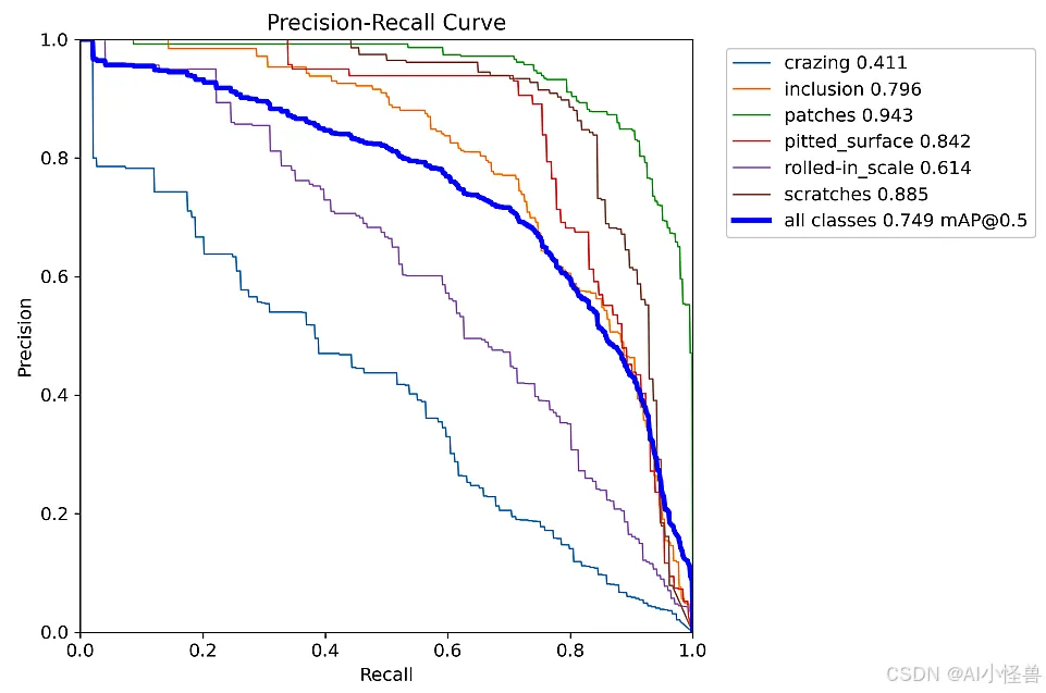

YOLOv13n-MSCA1 summary: 562 layers, 2,584,809 parameters, 0 gradients, 6.5 GFLOPs
                 Class     Images  Instances      Box(P          R      mAP50      mAP75  mAP50-95): 100%|██████████| 16/16 [00:12<00:00,  1.32it/s]
                   all        486       1069      0.723      0.664      0.749      0.434      0.425
               crazing         69        149      0.654      0.191      0.411     0.0788      0.145
             inclusion         87        222      0.701      0.734      0.796      0.417      0.422
               patches         92        243      0.812      0.914      0.943      0.668      0.604
        pitted_surface         93        130      0.875      0.754      0.842      0.595      0.563
       rolled-in_scale         81        171      0.591      0.532      0.614      0.237      0.279
             scratches         90        154      0.704      0.857      0.885      0.605      0.535

4.2.3 yolov13-MSCA2.yaml
nc: 80 # number of classes
scales: # model compound scaling constants, i.e. 'model=yolov13n.yaml' will call yolov13.yaml with scale 'n'
  # [depth, width, max_channels]
  n: [0.50, 0.25, 1024]   # Nano
  s: [0.50, 0.50, 1024]   # Small
  l: [1.00, 1.00, 512]    # Large
  x: [1.00, 1.50, 512]    # Extra Large
backbone:
  # [from, repeats, module, args]
  - [-1, 1, Conv,  [64, 3, 2]] # 0-P1/2
  - [-1, 1, Conv,  [128, 3, 2, 1, 2]] # 1-P2/4
  - [-1, 2, DSC3k2,  [256, False, 0.25]]
  - [-1, 1, Conv,  [256, 3, 2, 1, 4]] # 3-P3/8
  - [-1, 2, DSC3k2,  [512, False, 0.25]]
  - [-1, 1, DSConv,  [512, 3, 2]] # 5-P4/16
  - [-1, 4, A2C2f, [512, True, 4]]
  - [-1, 1, DSConv,  [1024, 3, 2]] # 7-P5/32
  - [-1, 4, A2C2f, [1024, True, 1]] # 8
head:
  - [[4, 6, 8], 2, HyperACE, [512, 8, True, True, 0.5, 1, "both"]]
  - [-1, 1, nn.Upsample, [None, 2, "nearest"]]
  - [ 9, 1, DownsampleConv, []]
  - [[6, 9], 1, FullPAD_Tunnel, []]  #12
  - [[4, 10], 1, FullPAD_Tunnel, []]  #13
  - [[8, 11], 1, FullPAD_Tunnel, []] #14

  - [-1, 1, nn.Upsample, [None, 2, "nearest"]]
  - [[-1, 12], 1, Concat, [1]] # cat backbone P4
  - [-1, 2, DSC3k2, [512, True]] # 17
  - [[-1, 9], 1, FullPAD_Tunnel, []]  #18
  - [17, 1, nn.Upsample, [None, 2, "nearest"]]
  - [[-1, 13], 1, Concat, [1]] # cat backbone P3
  - [-1, 2, DSC3k2, [256, True]] # 21
  - [10, 1, Conv, [256, 1, 1]]
  - [[21, 22], 1, FullPAD_Tunnel, []]  #23

  - [-1, 1, Conv, [256, 3, 2]]
  - [[-1, 18], 1, Concat, [1]] # cat head P4
  - [-1, 2, DSC3k2, [512, True]] # 26
  - [[-1, 9], 1, FullPAD_Tunnel, []]
  - [26, 1, Conv, [512, 3, 2]]
  - [[-1, 14], 1, Concat, [1]] # cat head P5
  - [-1, 2, DSC3k2, [1024,True]] # 30 (P5/32-large)
  - [[-1, 11], 1, FullPAD_Tunnel, []]


  - [23, 1, MSCAAttention, []] # 32
  - [27, 1, MSCAAttention, []] # 33
  - [31, 1, MSCAAttention, []] # 34

  - [[32, 33, 34], 1, Detect, [nc]] # Detect(P3, P4, P5)

原始mAP50为0.742提升至0.749
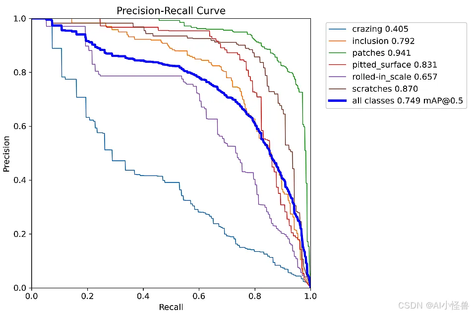

YOLOv13n-MSCA2 summary: 562 layers, 2,584,809 parameters, 0 gradients, 6.5 GFLOPs
                 Class     Images  Instances      Box(P          R      mAP50      mAP75  mAP50-95): 100%|██████████| 16/16 [00:12<00:00,  1.30it/s]
                   all        486       1069      0.735      0.685      0.749      0.418      0.424
               crazing         69        149      0.651      0.195      0.405     0.0783      0.149
             inclusion         87        222      0.727      0.752      0.792      0.392      0.435
               patches         92        243      0.823        0.9      0.941       0.71      0.612
        pitted_surface         93        130      0.805      0.777      0.831      0.599      0.558
       rolled-in_scale         81        171      0.685      0.608      0.657      0.227      0.297
             scratches         90        154      0.718      0.875       0.87      0.504      0.496

