- 这产生以下输出:
...
Generation 19500: Loss = 0.04461
 --- Test Accuracy = 80.47%.
Generation 19550: Loss = 0.01171
Generation 19600: Loss = 0.06911
Generation 19650: Loss = 0.08629
Generation 19700: Loss = 0.05296
Generation 19750: Loss = 0.03462
Generation 19800: Loss = 0.03182
Generation 19850: Loss = 0.07092
Generation 19900: Loss = 0.11342
Generation 19950: Loss = 0.08751
Generation 20000: Loss = 0.02228
 --- Test Accuracy = 83.59%.
- 最后,这里有一些
matplotlib代码将绘制在训练过程中的损失和测试准确率:
eval_indices = range(0, generations, eval_every)
output_indices = range(0, generations, output_every)
# Plot loss over time
plt.plot(output_indices, train_loss, 'k-')
plt.title('Softmax Loss per Generation')
plt.xlabel('Generation')
plt.ylabel('Softmax Loss')
plt.show()
# Plot accuracy over time
plt.plot(eval_indices, test_accuracy, 'k-')
plt.title('Test Accuracy')
plt.xlabel('Generation')
plt.ylabel('Accuracy')
plt.show()
我们得到以下秘籍的以下绘图:
[外链图片转存失败,源站可能有防盗链机制,建议将图片保存下来直接上传(img-XmuZWlzO-1681566911071)(https://gitcode.net/apachecn/apachecn-dl-zh/-/raw/master/docs/tf-ml-cookbook-2e-zh/img/8c38465a-ddc7-4389-9cc5-806b5a388769.png)]
图 5:训练损失在左侧,测试精度在右侧。对于 CIFAR-10 图像识别 CNN,我们能够实现在测试集上达到约 75% 准确率的模型
工作原理
在我们下载了 CIFAR-10 数据之后,我们建立了一个图像管道而不是使用源字典。有关图像管道的更多信息,请参阅 TensorFlow CIFAR-10 官方教程。我们使用此训练和测试管道来尝试预测图像的正确类别。最后,该模型在测试集上达到了约 75% 的准确率。
另见
- 有关 CIFAR-10 数据集的更多信息,请参阅学习 Tiny Images 的多个特征层,Alex Krizhevsky,2009
- 要查看原始的 TensorFlow 代码,请参阅此链接
- 有关局部响应归一化的更多信息,请参阅使用深度卷积神经网络的 ImageNet 分类,Krizhevsky,A. 等人,2012
重新训练现有的 CNN 模型
从头开始训练新的图像识别需要大量的时间和计算能力。如果我们可以采用先前训练的网络并使用我们的图像重新训练它,它可以节省我们的计算时间。对于此秘籍,我们将展示如何使用预先训练的 TensorFlow 图像识别模型并对其进行微调以处理不同的图像集。
准备
其思想是从卷积层重用先前模型的权重和结构,并重新训练网络顶部的完全连接层。
TensorFlow 在现有 CNN 模型的基础上创建了一个关于训练的教程(请参阅下一节中的第一个要点)。在本文中,我们将说明如何对 CIFAR-10 使用相同的方法。我们将采用的 CNN 网络使用一种非常流行的架构,称为 Inception。 Inception CNN 模型由 Google 创建,在许多图像识别基准测试中表现非常出色。有关详细信息,请参阅“另见”部分的第二个要点中的纸张参考。
我们将介绍的主要 Python 脚本显示如何下载 CIFAR-10 图像数据并自动分离,标记和保存图像到每个训练和测试文件夹中的十个类。之后,我们将重申如何在我们的图像上训练网络。
操作步骤
执行以下步骤:
- 我们首先加载必要的库来下载,解压缩和保存 CIFAR-10 图像:
import os
import tarfile
import _pickle as cPickle
import numpy as np
import urllib.request
import scipy.misc
from imageio import imwrite
- 我们现在声明 CIFAR-10 数据链接并创建我们将存储数据的临时目录。我们还将在以后保存图像时声明要引用的十个类别:
cifar_link = 'https://www.cs.toronto.edu/~kriz/cifar-10-python.tar.gz'
data_dir = 'temp'
if not os.path.isdir(data_dir):
    os.makedirs(data_dir)
objects = ['airplane', 'automobile', 'bird', 'cat', 'deer', 'dog', 'frog', 'horse', 'ship', 'truck']
- 现在我们将下载 CIFAR-10
.tar数据文件,并解压该文件:
target_file = os.path.join(data_dir, 'cifar-10-python.tar.gz')
if not os.path.isfile(target_file):
    print('CIFAR-10 file not found. Downloading CIFAR data (Size = 163MB)')
    print('This may take a few minutes, please wait.')
    filename, headers = urllib.request.urlretrieve(cifar_link, target_file)
# Extract into memory
tar = tarfile.open(target_file)
tar.extractall(path=data_dir)
tar.close()
- 我们现在为训练创建必要的文件夹结构。临时目录将有两个文件夹,
train_dir和validation_dir。在每个文件夹中,我们将为每个类别创建 10 个子文件夹:
# Create train image folders
train_folder = 'train_dir'
if not os.path.isdir(os.path.join(data_dir, train_folder)):
    for i in range(10):
        folder = os.path.join(data_dir, train_folder, objects[i])
        os.makedirs(folder)
# Create test image folders
test_folder = 'validation_dir'
if not os.path.isdir(os.path.join(data_dir, test_folder)):
    for i in range(10):
        folder = os.path.join(data_dir, test_folder, objects[i])
        os.makedirs(folder)
- 为了保存图像,我们将创建一个从内存加载它们并将它们存储在图像字典中的函数:
def load_batch_from_file(file):
    file_conn = open(file, 'rb')
    image_dictionary = cPickle.load(file_conn, encoding='latin1')
    file_conn.close()
    return(image_dictionary)
- 使用前面的字典,我们将使用以下函数将每个文件保存在正确的位置:
def save_images_from_dict(image_dict, folder='data_dir'):
    for ix, label in enumerate(image_dict['labels']):
        folder_path = os.path.join(data_dir, folder, objects[label])
        filename = image_dict['filenames'][ix]
        #Transform image data
        image_array = image_dict['data'][ix]
        image_array.resize([3, 32, 32])
        # Save image
        output_location = os.path.join(folder_path, filename)
        imwrite(output_location,image_array.transpose())
- 使用上述函数,我们可以遍历下载的数据文件并将每个图像保存到正确的位置:
data_location = os.path.join(data_dir, 'cifar-10-batches-py')
train_names = ['data_batch_' + str(x) for x in range(1,6)]
test_names = ['test_batch']
# Sort train images
for file in train_names:
    print('Saving images from file: {}'.format(file))
    file_location = os.path.join(data_dir, 'cifar-10-batches-py', file)
    image_dict = load_batch_from_file(file_location)
    save_images_from_dict(image_dict, folder=train_folder)
# Sort test images
for file in test_names:
    print('Saving images from file: {}'.format(file))
    file_location = os.path.join(data_dir, 'cifar-10-batches-py', file)
    image_dict = load_batch_from_file(file_location)
    save_images_from_dict(image_dict, folder=test_folder)
- 我们脚本的最后一部分创建了图像标签文件,这是我们需要的最后一条信息。这个文件让我们将输出解释为标签而不是数字索引:
cifar_labels_file = os.path.join(data_dir,'cifar10_labels.txt')
print('Writing labels file, {}'.format(cifar_labels_file))
with open(cifar_labels_file, 'w') as labels_file:
    for item in objects:
        labels_file.write("{}n".format(item))
- 当前面的脚本运行时,它将下载图像并将它们分类到 TensorFlow 再训练教程所期望的正确文件夹结构中。完成后,我们只需按照教程进行操作即可。首先,我们应该克隆教程仓库:
git clone https://github.com/tensorflow/models/tree/master/research/inception
- 为了使用先前训练的模型,我们必须下载网络权重并将其应用于我们的模型。为此,您必须访问该站点,并按照说明下载并安装 cifar10 模型架构和权重。您还将最终下载包含下面描述的构建,训练和测试脚本的数据目录。
对于此步骤,我们导航到
research/inception/inception目录,然后执行以下命令,--train_directory,--validation_directory,--output_directory和--labels_file的路径指向相对路径或完整路径创建的目录结构。
- 现在我们将图像放在正确的文件夹结构中,我们必须将它们变成
TFRecords对象。我们通过运行以下命令来完成此操作:
me@computer:~$ python3 data/build_image_data.py
    --train_directory="temp/train_dir/"
    --validation_directory="temp/validation_dir"
    --output_directory="temp/" --labels_file="temp/cifar10_labels.txt"
- 现在我们将使用
bazel训练模型,将参数设置为true。该脚本每 10 代输出一次损失。我们可以随时终止此过程,模型输出将在temp/training_results文件夹中。我们可以从此文件夹加载模型以进行评估:
me@computer:~$ bazel-bin/inception/flowers_train
    --train_dir="temp/training_results" --data_dir="temp/data_dir"
    --pretrained_model_checkpoint_path="model.ckpt-157585"
    --fine_tune=True --initial_learning_rate=0.001
    --input_queue_memory_factor=1
- 这应该使输出类似于以下内容:
2018-06-02 11:10:10.557012: step 1290, loss = 2.02 (1.2  examples/sec; 23.771 sec/batch)
...
工作原理
关于预训练 CNN 上的训练的 TensorFlow 官方教程需要设置一个文件夹;我们从 CIFAR-10 数据创建的设置。然后我们将数据转换为所需的TFRecords格式并开始训练模型。请记住,我们正在微调模型并重新训练顶部的完全连接的层以适合我们的 10 类数据。
另见
应用 StyleNet 和 NeuralStyle 项目
一旦我们对 CNN 进行了图像识别训练,我们就可以将网络本身用于一些有趣的数据和图像处理。 Stylenet 是一种尝试从一张图片中学习图像样式并将其应用于第二张图片同时保持第二图像结构(或内容)完整的过程。如果我们能够找到与样式强烈相关的中间 CNN 节点,这可能是可能的,与图像的内容分开。
准备
Stylenet 是一个过程,它接收两个图像并将一个图像的样式应用于第二个图像的内容。它基于 2015 年的着名论文“艺术风格的神经算法”(参见下一节的第一个要点)。作者在一些 CNN 中找到了一个属性,其中存在中间层,它们似乎编码图片的样式,有些编码图片的内容。为此,如果我们训练样式图片上的样式层和原始图像上的内容层,并反向传播那些计算的损失,我们可以将原始图像更改为更像样式图像。
为了实现这一目标,我们将下载本文推荐的网络;叫做 imagenet-vgg-19。还有一个 imagenet-vgg-16 网络也可以使用,但是本文推荐使用 imagenet-vgg-19。
操作步骤
执行以下步骤:
- 首先,我们将以
mat格式下载预先训练好的网络。mat格式是matlab对象,Python 中的scipy包有一个可以读取它的方法。下载mat对象的链接在这里。我们将此模型保存在 Python 脚本所在的同一文件夹中,以供参考:
http://www.vlfeat.org/matconvnet/models/beta16/imagenet-vgg-verydeep-19.mat
- 我们将通过加载必要的库来启动我们的 Python 脚本:
import os
import scipy.io
import scipy.misc
import imageio
from skimage.transform import resize
from operator import mul
from functools import reduce
import numpy as np
import tensorflow as tf
from tensorflow.python.framework import ops
ops.reset_default_graph()
- 然后我们可以声明两个图像的位置:原始图像和样式图像。出于我们的目的,我们将使用本书的封面图片作为原始图像;对于风格形象,我们将使用文森特·梵高的星夜。随意使用您想要的任何两张图片。如果您选择使用这些图片,可以在本书的 GitHub 网站上找到(导航到 Styelnet 部分):
original_image_file = 'temp/book_cover.jpg'
style_image_file = 'temp/starry_night.jpg'
- 我们将为我们的模型设置一些参数:
mat文件的位置,权重,学习率,代数以及输出中间图像的频率。对于权重,有助于在原始图像上高度加权样式图像。应根据所需结果的变化调整这些超参数:
vgg_path = 'imagenet-vgg-verydeep-19.mat'
original_image_weight = 5.0
style_image_weight = 500.0
regularization_weight = 100
learning_rate = 10
generations = 100
output_generations = 25
beta1 = 0.9
beta2 = 0.999
- 现在我们将使用
scipy加载两个图像并更改样式图像以适合原始图像大小:
original_image = imageio.imread(original_image_file)
style_image = imageio.imread(style_image_file)
# Get shape of target and make the style image the same
target_shape = original_image.shape
style_image = resize(style_image, target_shape)
- 从论文中,我们可以按照它们出现的顺序定义层。我们将使用作者的命名约定:
vgg_layers = ['conv1_1', 'relu1_1',
              'conv1_2', 'relu1_2', 'pool1',
              'conv2_1', 'relu2_1',
              'conv2_2', 'relu2_2', 'pool2',
              'conv3_1', 'relu3_1',
              'conv3_2', 'relu3_2',
              'conv3_3', 'relu3_3',
              'conv3_4', 'relu3_4', 'pool3',
              'conv4_1', 'relu4_1',
              'conv4_2', 'relu4_2',
              'conv4_3', 'relu4_3',
              'conv4_4', 'relu4_4', 'pool4',
              'conv5_1', 'relu5_1',
              'conv5_2', 'relu5_2',
              'conv5_3', 'relu5_3',
              'conv5_4', 'relu5_4']
- 现在我们将定义一个从
mat文件中提取参数的函数:
def extract_net_info(path_to_params):
    vgg_data = scipy.io.loadmat(path_to_params)
    normalization_matrix = vgg_data['normalization'][0][0][0]
    mat_mean = np.mean(normalization_matrix, axis=(0,1))
    network_weights = vgg_data['layers'][0]
    return mat_mean, network_weights
- 根据加载的权重和
layer定义,我们可以使用以下函数在 TensorFlow 中重新创建网络。我们将遍历每一层并使用适当的weights和biases分配相应的函数,如果适用:
def vgg_network(network_weights, init_image):
    network = {}
    image = init_image
    for i, layer in enumerate(vgg_layers):
        if layer[1] == 'c':
            weights, bias = network_weights[i][0][0][0][0]
            weights = np.transpose(weights, (1, 0, 2, 3))
            bias = bias.reshape(-1)
            conv_layer = tf.nn.conv2d(image, tf.constant(weights), (1, 1, 1, 1), 'SAME')
            image = tf.nn.bias_add(conv_layer, bias)
        elif layer[1] == 'r':
            image = tf.nn.relu(image)
        else:
            image = tf.nn.max_pool(image, (1, 2, 2, 1), (1, 2, 2, 1), 'SAME')
        network[layer] = image
    return(network)
- 本文推荐了一些策略,用于将中间层分配给原始图像和样式图像。虽然我们应该为原始图像保留
relu4_2,但我们可以为样式图像尝试其他reluX_1层输出的不同组合:
original_layer = ['relu4_2']
style_layers = ['relu1_1', 'relu2_1', 'relu3_1', 'relu4_1', 'relu5_1']
- 接下来,我们将运行前面的函数来获取权重和均值。我们还需要均匀设置 VGG19 样式层权重。如果您愿意,可以通过更改权重进行实验。现在,我们假设它们对于两个层都是 0.5:
# Get network parameters
normalization_mean, network_weights = extract_net_info(vgg_path)
shape = (1,) + original_image.shape
style_shape = (1,) + style_image.shape
original_features = {}
style_features = {}
# Set style weights
style_weights = {l: 1./(len(style_layers)) for l in style_layers}
- 为了忠实于原始图片外观,我们希望添加一个损失值,将内容/原始特征与原始内容特征进行比较。为此,我们加载 VGG19 模型并计算原始内容特征的内容/原始特征:
g_original = tf.Graph()
with g_original.as_default(), tf.Session() as sess1:
    image = tf.placeholder('float', shape=shape)
    vgg_net = vgg_network(network_weights, image)
    original_minus_mean = original_image - normalization_mean
    original_norm = np.array([original_minus_mean])
    for layer in original_layers:
        original_features[layer] = vgg_net[layer].eval(feed_dict={image: original_norm})
- 与步骤 11 类似,我们希望将原始图像的样式特征更改为样式图片的样式特征。为此,我们将为损失函数添加样式损失值。此损失值需要查看我们预先确定的样式层中样式图像的值。我们还将通过单独的图运行此操作。我们按如下方式计算这些样式特征:
# Get style image network
g_style = tf.Graph()
with g_style.as_default(), tf.Session() as sess2:
    image = tf.placeholder('float', shape=style_shape)
    vgg_net = vgg_network(network_weights, image)
    style_minus_mean = style_image - normalization_mean
    style_norm = np.array([style_minus_mean])
    for layer in style_layers:
        features = vgg_net[layer].eval(feed_dict={image: style_norm})
        features = np.reshape(features, (-1, features.shape[3]))
        gram = np.matmul(features.T, features) / features.size
        style_features[layer] = gram
- 我们启动默认图来计算损失和训练步骤。首先,我们首先将随机图像初始化为 TensorFlow 变量:
# Make Combined Image via loss function
with tf.Graph().as_default():
    # Get network parameters
    initial = tf.random_normal(shape) * 0.256
    init_image = tf.Variable(initial)
    vgg_net = vgg_network(network_weights, init_image)
- 接下来,我们计算原始内容损失(将其缩进到默认图下)。这个损失部分将尽可能保持原始图像的结构完整:
# Loss from Original Image
original_layers_w = {'relu4_2': 0.5, 'relu5_2': 0.5}
original_loss = 0
for o_layer in original_layers:
    temp_original_loss = original_layers_w[o_layer] * original_image_weight *\
                (2 * tf.nn.l2_loss(vgg_net[o_layer] - original_features[o_layer]))
    original_loss += (temp_original_loss / original_features[o_layer].size)
- 仍然在默认图缩进下,我们创建第二个损失项,即样式损失。此损失将比较我们预先计算的样式特征与输入图像的样式特征(随机初始化):
# Loss from Style Image
style_loss = 0
style_losses = []
for style_layer in style_layers:
    layer = vgg_net[style_layer]
    feats, height, width, channels = [x.value for x in layer.get_shape()]
    size = height * width * channels
    features = tf.reshape(layer, (-1, channels))
    style_gram_matrix = tf.matmul(tf.transpose(features), features) / size
    style_expected = style_features[style_layer]
    style_losses.append(style_weights[style_layer] * 2 *
                        tf.nn.l2_loss(style_gram_matrix - style_expected) /
                        style_expected.size)
style_loss += style_image_weight * tf.reduce_sum(style_losses)
- 第三个也是最后一个损失条款将有助于平滑图像。我们在这里使用总变差损失来惩罚相邻像素的剧烈变化,如下所示:
total_var_x = reduce(mul, init_image[:, 1:, :, :].get_shape().as_list(), 1)
total_var_y = reduce(mul, init_image[:, :, 1:, :].get_shape().as_list(), 1)
first_term = regularization_weight * 2
second_term_numerator = tf.nn.l2_loss(init_image[:, 1:, :, :] - init_image[:, :shape[1]-1, :, :])
second_term = second_term_numerator / total_var_y
third_term = (tf.nn.l2_loss(init_image[:, :, 1:, :] - init_image[:, :, :shape[2]-1, :]) / total_var_x)
total_variation_loss = first_term * (second_term + third_term)
- 接下来,我们结合损失项并创建优化函数和训练步骤,如下所示:
# Combined Loss
loss = original_loss + style_loss + total_variation_loss
# Declare Optimization Algorithm
optimizer = tf.train.AdamOptimizer(learning_rate, beta1, beta2)
train_step = optimizer.minimize(loss)
- 现在我们运行训练步骤,保存中间图像,并保存最终输出图像,如下所示:
# Initialize variables and start training
with tf.Session() as sess:
    tf.global_variables_initializer().run()
    for i in range(generations):
        train_step.run()
        # Print update and save temporary output
        if (i+1) % output_generations == 0:
            print('Generation {} out of {}, loss: {}'.format(i + 1, generations, sess.run(loss)))
            image_eval = init_image.eval()
            best_image_add_mean = image_eval.reshape(shape[1:]) + normalization_mean
            output_file = 'temp_output_{}.jpg'.format(i)
            imageio.imwrite(output_file, best_image_add_mean.astype(np.uint8))
    # Save final image
    image_eval = init_image.eval()
    best_image_add_mean = image_eval.reshape(shape[1:]) + normalization_mean
    output_file = 'final_output.jpg'
    scipy.misc.imsave(output_file, best_image_add_mean)
[外链图片转存失败,源站可能有防盗链机制,建议将图片保存下来直接上传(img-g3DnfZUm-1681566911072)(https://gitcode.net/apachecn/apachecn-dl-zh/-/raw/master/docs/tf-ml-cookbook-2e-zh/img/f26567a0-ae26-409e-87ee-2ef19c33567d.png)]
图 6:使用 Stylenet 算法将书籍封面图像与星夜相结合。请注意,可以通过更改脚本开头的权重来使用不同的样式重点
工作原理
我们首先加载两个图像,然后将预先训练的网络权重和指定的层加载到原始图像和样式图像。我们计算了三种损失函数:原始图像损失,样式损失和总变差损失。然后我们训练随机噪声图片以使用样式图像的样式和原始图像的内容。
损失函数受 GitHub 神经风格项目的影响很大。我们还强烈建议读者查看这些项目中的代码以获得改进,更多细节,以及通常更强大的算法,可以提供更好的结果。
另见
- Gatys,Ecker,Bethge 的艺术风格神经算法,2015
- Leon Gatys 在 CVPR 2016(计算机视觉和模式识别)上的一个很好的推荐视频
实现 DeepDream
受过训练的 CNN 的另一个用途是利用一些中间节点检测标签特征(例如,猫的耳朵或鸟的羽毛)的事实。利用这一事实,我们可以找到转换任何图像的方法,以反映我们选择的任何节点的节点特征。对于这个秘籍,我们将在 TensorFlow 的网站上浏览 DeepDream 教程,但我们将更详细地介绍基本部分。希望我们可以让读者准备好使用 DeepDream 算法来探索 CNN 及其中创建的特征。
准备
TensorFlow 的官方教程展示了如何通过脚本实现 DeepDream(请参阅下一节中的第一个要点)。这个方法的目的是通过他们提供的脚本并解释每一行。虽然教程很棒,但有些部分可以跳过,有些部分可以使用更多解释。我们希望提供更详细的逐行说明。我们还将在必要时使代码符合 Python3 标准。
操作步骤
执行以下步骤:
- 为了开始使用 DeepDream,我们需要下载在 CIFAR-1000 上接受过 CNN 训练的 GoogleNet:
me@computer:~$ wget https://storage.googleapis.com/download.tensorflow.org/models/inception5h.zip
me@computer:~$ unzip inception5h.zip
- 我们首先加载必要的库并启动图会话:
import os
import matplotlib.pyplot as plt
import numpy as np
import PIL.Image
import tensorflow as tf
from io import BytesIO
graph = tf.Graph()
sess = tf.InteractiveSession(graph=graph)
- 我们现在声明解压缩模型参数的位置(从步骤 1 开始)并将参数加载到 TensorFlow 图中:
# Model location
model_fn = 'tensorflow_inception_graph.pb'
# Load graph parameters
with tf.gfile.FastGFile(model_fn, 'rb') as f:
    graph_def = tf.GraphDef()
    graph_def.ParseFromString(f.read())
- 我们为输入创建一个占位符,保存 imagenet 平均值 117.0,然后使用正则化占位符导入图定义:
# Create placeholder for input
t_input = tf.placeholder(np.float32, name='input')
# Imagenet average bias to subtract off images
imagenet_mean = 117.0
t_preprocessed = tf.expand_dims(t_input-imagenet_mean, 0)
tf.import_graph_def(graph_def, {'input':t_preprocessed})
- 接下来,我们将导入卷积层,以便在以后可视化并使用它们进行 DeepDream 处理:
# Create a list of layers that we can refer to later
layers = [op.name for op in graph.get_operations() if op.type=='Conv2D' and 'import/' in op.name]
# Count how many outputs for each layer
feature_nums = [int(graph.get_tensor_by_name(name+':0').get_shape()[-1]) for name in layers]
- 现在我们将选择一个可视化的层。我们也可以通过名字选择其他人。我们选择查看特征号
139。图像以随机噪声开始:
layer = 'mixed4d_3x3_bottleneck_pre_relu'
channel = 139
img_noise = np.random.uniform(size=(224,224,3)) + 100.0
- 我们声明了一个绘制图像数组的函数:
def showarray(a, fmt='jpeg'):
    # First make sure everything is between 0 and 255
    a = np.uint8(np.clip(a, 0, 1)*255)
    # Pick an in-memory format for image display
    f = BytesIO()
    # Create the in memory image
    PIL.Image.fromarray(a).save(f, fmt)
    # Show image
    plt.imshow(a)
- 我们将通过创建一个从图中按名称检索层的函数来缩短一些重复代码:
def T(layer): #Helper for getting layer output tensor return graph.get_tensor_by_name("import/%s:0"%layer)
- 我们将创建的下一个函数是一个包装函数,用于根据我们指定的参数创建占位符:
# The following function returns a function wrapper that will create the placeholder
# inputs of a specified dtype
def tffunc(*argtypes):
    '''Helper that transforms TF-graph generating function into a regular one.
    See "resize" function below.
    '''
    placeholders = list(map(tf.placeholder, argtypes))
    def wrap(f):
        out = f(*placeholders)
        def wrapper(*args, **kw):
            return out.eval(dict(zip(placeholders, args)), session=kw.get('session'))
        return wrapper
    return wrap
- 我们还需要一个将图像大小调整为大小规格的函数。我们使用 TensorFlow 的内置图像线性插值函数:
tf.image.resize.bilinear()
# Helper function that uses TF to resize an image
def resize(img, size):
    img = tf.expand_dims(img, 0)
    # Change 'img' size by linear interpolation
    return tf.image.resize_bilinear(img, size)[0,:,:,:]
- 现在我们需要一种方法来更新源图像,使其更像我们使用的特征。我们通过指定如何计算图像上的梯度来完成此操作。我们定义了一个函数,用于计算图像上子区域(图块)的梯度,以加快计算速度。为了防止平铺输出,我们将在
x和y方向上随机移动或滚动图像,这将平滑平铺效果:
def calc_grad_tiled(img, t_grad, tile_size=512):
    '''Compute the value of tensor t_grad over the image in a tiled way.
    Random shifts are applied to the image to blur tile boundaries over
    multiple iterations.'''
    # Pick a subregion square size
    sz = tile_size
    # Get the image height and width
    h, w = img.shape[:2]
    # Get a random shift amount in the x and y direction
    sx, sy = np.random.randint(sz, size=2)
    # Randomly shift the image (roll image) in the x and y directions
    img_shift = np.roll(np.roll(img, sx, 1), sy, 0)
    # Initialize the while image gradient as zeros
    grad = np.zeros_like(img)
    # Now we loop through all the sub-tiles in the image
    for y in range(0, max(h-sz//2, sz),sz):
        for x in range(0, max(w-sz//2, sz),sz):
            # Select the sub image tile
            sub = img_shift[y:y+sz,x:x+sz]
            # Calculate the gradient for the tile
            g = sess.run(t_grad, {t_input:sub})
            # Apply the gradient of the tile to the whole image gradient
            grad[y:y+sz,x:x+sz] = g
    # Return the gradient, undoing the roll operation
    return np.roll(np.roll(grad, -sx, 1), -sy, 0)
- 现在我们可以声明 DeepDream 函数。我们算法的目标是我们选择的特征的平均值。损耗在梯度上运行,这取决于输入图像和所选特征之间的距离。策略是将图像分成高频和低频,并计算低频部分的梯度。将得到的高频图像再次分开并重复该过程。原始图像和低频图像的集合称为
octaves。对于每次传递,我们计算梯度并将它们应用于图像:
def render_deepdream(t_obj, img0=img_noise,
                     iter_n=10, step=1.5, octave_n=4, octave_scale=1.4):
    # defining the optimization objective, the objective is the mean of the feature
    t_score = tf.reduce_mean(t_obj)
    # Our gradients will be defined as changing the t_input to get closer to the values of t_score.  Here, t_score is the mean of the feature we select.
    # t_input will be the image octave (starting with the last)
    t_grad = tf.gradients(t_score, t_input)[0] # behold the power of automatic differentiation!
    # Store the image
    img = img0
    # Initialize the image octave list
    octaves = []
    # Since we stored the image, we need to only calculate n-1 octaves
    for i in range(octave_n-1):
        # Extract the image shape
        hw = img.shape[:2]
        # Resize the image, scale by the octave_scale (resize by linear interpolation)
        lo = resize(img, np.int32(np.float32(hw)/octave_scale))
        # Residual is hi.  Where residual = image - (Resize lo to be hw-shape)
        hi = img-resize(lo, hw)
        # Save the lo image for re-iterating
        img = lo
        # Save the extracted hi-image
        octaves.append(hi)
    # generate details octave by octave
    for octave in range(octave_n):
        if octave>0:
            # Start with the last octave
            hi = octaves[-octave]
            #
            img = resize(img, hi.shape[:2])+hi
        for i in range(iter_n):
            # Calculate gradient of the image.
            g = calc_grad_tiled(img, t_grad)
            # Ideally, we would just add the gradient, g, but
            # we want do a forward step size of it ('step'),
            # and divide it by the avg. norm of the gradient, so
            # we are adding a gradient of a certain size each step.
            # Also, to make sure we aren't dividing by zero, we add 1e-7\.
            img += g*(step / (np.abs(g).mean()+1e-7))
            print('.',end = ' ')
        showarray(https://gitcode.net/apachecn/apachecn-dl-zh/-/raw/master/docs/tf-ml-cookbook-2e-zh/img/255.0)
- 通过我们所做的所有特征设置,我们现在可以运行 DeepDream 算法:
# Run Deep Dream
if __name__=="__main__":
    # Create resize function that has a wrapper that creates specified placeholder types
    resize = tffunc(np.float32, np.int32)(resize)
    # Open image
    img0 = PIL.Image.open('book_cover.jpg')
    img0 = np.float32(img0)
    # Show Original Image
    showarray(img0/255.0)
    # Create deep dream
    render_deepdream(T(layer)[:,:,:,139], img0, iter_n=15)
    sess.close()
输出如下:
[外链图片转存失败,源站可能有防盗链机制,建议将图片保存下来直接上传(img-0JlWV3VB-1681566911072)(https://gitcode.net/apachecn/apachecn-dl-zh/-/raw/master/docs/tf-ml-cookbook-2e-zh/img/07fcab05-6c73-4aeb-b2ed-a1330c65fa0d.png)]
图 7:本书的封面,贯穿 DeepDream 算法,其特征层编号为 50,110,100 和 139
更多
我们敦促读者使用 DeepDream 官方教程作为进一步信息的来源,并访问 DeepDream 上的原始 Google 研究博客文章(请参阅下面的第二个要点参见另见部分)。