在分类问题中,预测准确度如果简单的用预测成功的概率来代表的话,有时候即使得到了99.9%的准确率,也不一定说明模型和算法就是好的,例如癌症问题,假如癌症的发病率只有0.01%,那么如果算法始终给出不得病的预测结果,也能达到很高的准确率
混淆矩阵
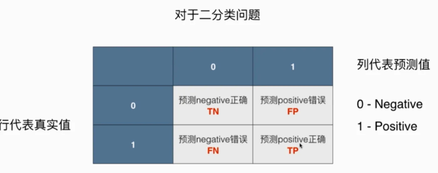
二分类问题的混淆矩阵
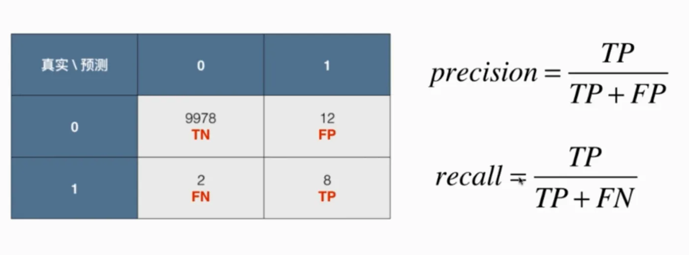
以癌症为例,0代表未患病,1代表患病,有10000个人:
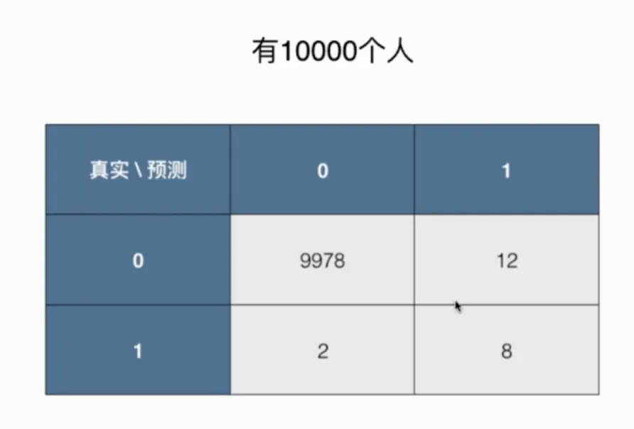
癌症问题的混淆矩阵
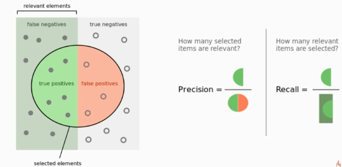
精准率和召唤率
代码实现
#准备数据
import numpy as np
from sklearn import datasets

digits = datasets.load_digits()
X = digits['data']
y = digits['target'].copy()

#手动让digits数据集9的数据偏斜
y[digits['target']==9] = 1
y[digits['target']!=9] = 0

from sklearn.linear_model import LogisticRegression
from sklearn.model_selection import train_test_split

X_train,X_test,y_train,y_test = train_test_split(X,y,random_state=666)

log_reg = LogisticRegression()
log_reg.fit(X_train,y_train)
log_reg.score(X_test,y_test)

y_log_predict = log_reg.predict(X_test)
def TN(y_true,y_predict):
    return np.sum((y_true==0)&(y_predict==0))
TN(y_test,y_log_predict)

def FP(y_true,y_predict):
    return np.sum((y_true==0)&(y_predict==1))
FP(y_test,y_log_predict)

def FN(y_true,y_predict):
    return np.sum((y_true==1)&(y_predict==0))
FN(y_test,y_log_predict)

def TP(y_true,y_predict):
    return np.sum((y_true==1)&(y_predict==1))
TP(y_test,y_log_predict)

#构建混淆矩阵
def confusion_matrix(y_true,y_predict):
    return np.array([
        [TN(y_true,y_predict),FP(y_true,y_predict)],
        [FN(y_true,y_predict),TP(y_true,y_predict)]
    ])
confusion_matrix(y_test,y_log_predict)

#精准率
def precision_score(y_true,y_predict):
    tp = TP(y_true,y_predict)
    fp = FP(y_true,y_predict)
    try:
        return tp/(tp+fp)
    except:
        return 0.0
precision_score(y_test,y_log_predict)

#召回率
def recall_score(y_true,y_predict):
    tp = TP(y_true,y_predict)
    fn = FN(y_true,y_predict)
    try:
        return tp/(tp+fn)
    except:
        return 0.0
recall_score(y_test,y_log_predict)
scikitlearn中的精准率和召回率
#构建混淆矩阵
from sklearn.metrics import confusion_matrix
confusion_matrix(y_test,y_log_predict)

#精准率
from sklearn.metrics import precision_score
precision_score(y_test,y_log_predict)
调和平均值F1_score
调和平均数具有以下几个主要特点:
①调和平均数易受极端值的影响,且受极小值的影响比受极大值的影响更大。
②只要有一个标志值为0,就不能计算调和平均数。

调用sikit-learn中的f1_score
from sklearn.metrics import f1_score
f1_score(y_test,y_log_predict)
>>> 0.86
Precision-Recall的平衡
 一般来说,决策边界为theta.T*x_b=0,即计算出p>0.5时分类为1,如果我们手动改变这个threshold,就可以平移这个决策边界,改变精准率和召回率
#该函数可以得到log_reg的预测分数,未带入sigmoid
decsion_scores = log_reg.decision_function(X_test)

#将threshold由默认的0调为5
y_predict2 = decsion_scores>=5.0
precision_score(y_test,y_predict2)
>>> 0.96
recall_score(y_test,y_predict2)
>>> 0.5333333333333333

y_predict2 = decsion_scores>=-5.0
precision_score(y_test,y_predict2)
>>> 0.7272727272727273
recall_score(y_test,y_predict2)
>>> 0.8888888888888888
精准率和召回率曲线
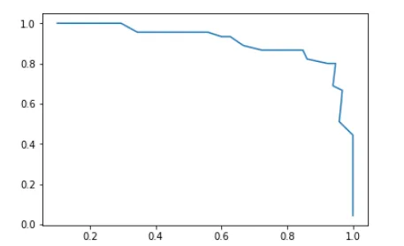
可以用precisions-recalls曲线与坐标轴围成的面积衡量模型的好坏
from sklearn.metrics import precision_score
from sklearn.metrics import recall_score

thresholds = np.arange(np.min(decsion_scores),np.max(decsion_scores))
precisions = []
recalls = []

for threshold in thresholds:
    y_predict = decsion_scores>=threshold
    precisions.append(precision_score(y_test,y_predict))
    recalls.append(recall_score(y_test,y_predict))
import matplotlib.pyplot as plt
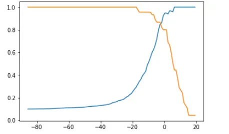
plt.plot(thresholds,precisions)
plt.plot(thresholds,recalls)
plt.show()
plt.plot(precisions,recalls)
plt.show()
使用scikit-learn绘制Precision-Recall曲线
from sklearn.metrics import precision_recall_curve
precisions,recalls,thresholds = precision_recall_curve(y_test,decsion_scores)

#由于precisions和recalls中比thresholds多了一个元素,因此要绘制曲线,先去掉这个元素
plt.plot(thresholds,precisions[:-1])
plt.plot(thresholds,recalls[:-1])
plt.show()
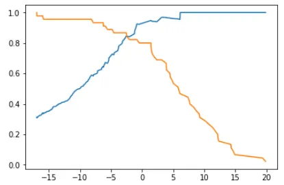
由于scikit-learn中对于shelods的取值和上面用到的不一样,因此曲线图像略有不同
ROC曲线
ROC曲线用于描述TPR和FPR之间的关系
 TPR定义
TPR定义 FPR定义
FPR定义
使用sikit-learn绘制ROC
from sklearn.metrics import roc_curve

fprs,tprs,thresholds = roc_curve(y_test,decsion_scores)
plt.plot(fprs,tprs)

横轴fpr,纵轴tpr
ROC曲线围成的面积越大,说明模型越好,不过ROC曲线没有Precision-Recall曲线那样对偏斜的数据的敏感性
多分类问题
#这次我们使用所有数据来进行逻辑回归的多分类问题的处理。
X = digits['data']
y = digits['target']
X_train,X_test,y_train,y_test = train_test_split(X,y)

log_reg = LogisticRegression()
log_reg.fit(X_train,y_train)
log_reg.score(X_test,y_test)
>>> 0.9577777777777777
scikit-learn中处理多分类问题的准确率
from sklearn.metrics import precision_score

#precision_score函数本身不能计算多分类问题,需要修改average参数
precision_score(y_test,y_predict,average='micro')
>>> 0.9577777777777777
多分类问题的混淆矩阵
多分类问题的混淆矩阵解读方式与二分类问题一致,第i行第j列的值就是真值为i、预测值为j的元素的数量
from sklearn.metrics import confusion_matrix

confusion_matrix(y_test,y_predict)
>>> array([[30,  0,  0,  0,  0,  0,  0,  1,  0,  0],
       [ 0, 43,  0,  2,  0,  0,  1,  0,  4,  0],
       [ 0,  0, 41,  0,  0,  0,  0,  0,  0,  0],
       [ 0,  0,  0, 47,  0,  0,  0,  0,  0,  1],
       [ 0,  0,  0,  0, 46,  0,  0,  0,  0,  2],
       [ 0,  0,  0,  0,  0, 51,  0,  0,  0,  1],
       [ 0,  0,  0,  0,  0,  0, 38,  0,  1,  0],
       [ 0,  0,  0,  0,  0,  0,  0, 58,  0,  0],
       [ 0,  1,  0,  1,  1,  0,  0,  0, 37,  0],
       [ 0,  1,  0,  1,  0,  0,  0,  0,  1, 40]], dtype=int64)
绘制混淆矩阵
cfm = confusion_matrix(y_test,y_predict)
#cmap参数为绘制矩阵的颜色集合,这里使用灰度
plt.matshow(cfm,cmap=plt.cm.gray)
plt.show()
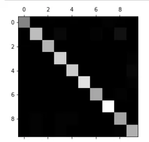
颜色越亮的地方代表数值越高
绘制错误率矩阵
#计算每一行的总值
row_sums = np.sum(cfm,axis=1)
err_matrix = cfm/row_sums
#对err_matrix矩阵的对角线置0,因为这是预测正确的部分,不关心
np.fill_diagonal(err_matrix,0)
err_matrix
>>> array([[0.        , 0.        , 0.        , 0.        , 0.        ,
        0.        , 0.        , 0.01724138, 0.        , 0.        ],
       [0.        , 0.        , 0.        , 0.04166667, 0.        ,
        0.        , 0.02564103, 0.        , 0.1       , 0.        ],
       [0.        , 0.        , 0.        , 0.        , 0.        ,
        0.        , 0.        , 0.        , 0.        , 0.        ],
       [0.        , 0.        , 0.        , 0.        , 0.        ,
        0.        , 0.        , 0.        , 0.        , 0.02325581],
       [0.        , 0.        , 0.        , 0.        , 0.        ,
        0.        , 0.        , 0.        , 0.        , 0.04651163],
       [0.        , 0.        , 0.        , 0.        , 0.        ,
        0.        , 0.        , 0.        , 0.        , 0.02325581],
       [0.        , 0.        , 0.        , 0.        , 0.        ,
        0.        , 0.        , 0.        , 0.025     , 0.        ],
       [0.        , 0.        , 0.        , 0.        , 0.        ,
        0.        , 0.        , 0.        , 0.        , 0.        ],
       [0.        , 0.02      , 0.        , 0.02083333, 0.02083333,
        0.        , 0.        , 0.        , 0.        , 0.        ],
       [0.        , 0.02      , 0.        , 0.02083333, 0.        ,
        0.        , 0.        , 0.        , 0.025     , 0.        ]])
plt.matshow(err_matrix,cmap=plt.cm.gray)
plt.show()
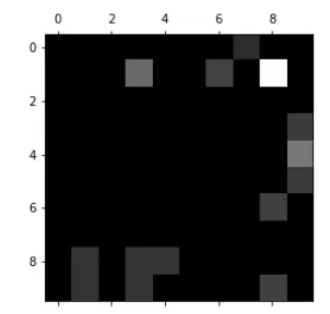
亮度越高的地方代表错误率越高