 1. 密度泛函理论
密度泛函理论(Density Functional Theory)是一种研究多电子体系电子结构的量子力学方法。密度泛函理论在物理和化学上都有广泛的应用,特别是用来研究分子和凝聚态的性质,是凝聚态物理和计算化学领域最常用的方法之一。
电子结构理论的经典方法,特别是Hartree-Fock方法和后Hartree-Fock方法,是基于复杂的多电子波函数的。密度泛函理论的主要目标就是用电子密度取代波函数做为研究的基本量。因为多电子波函数有3N个变量(N 为电子数,每个电子包含三个空间变量),而电子密度仅是三个变量的函数,无论在概念上还是实际上都更方便处理。
Hohenberg-Kohn定理为泛函理论提供了坚实的理论基础:
第一定理指出体系的基态能量仅仅是电子密度的泛函。
第二定理证明了以基态密度为变量,将体系能量通过变分得到最小值之后就得到了基态能量。
密度泛函理论最普遍的应用是通过Kohn-Sham方法实现的。在Kohn-Sham DFT框架中,最难处理的多体问题被简化成了一个没有相互作用的电子在有效势场中的运动问题。
2. Numpy 1D-DFT
http://dcwww.camd.dtu.dk/~askhl/files/python-dft-exercises.pdf
Goal: write our own Kohn-Sham (KS) DFT code
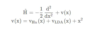
Target: a harmonic oscillator including kinetic energy, electrostatic repulsion between the electrons, and the local density approximation for electronic interactions, ignoring correlation.
Hamiltonian:
What we have to do?
- Represent the Hamiltonian
- Calculate the KS wavefunctions, the density
import numpy as np
import matplotlib.pyplot as plt
2.1 Differential operator
In order to represent kinetic operator
2.1.1 First order differentiation
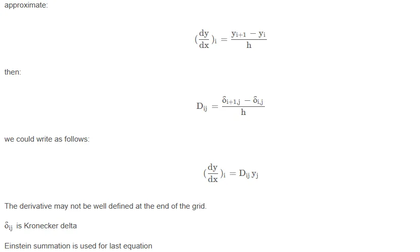
n_grid=200
x=np.linspace(-5,5,n_grid)
h=x[1]-x[0]
D=-np.eye(n_grid)+np.diagflat(np.ones(n_grid-1),1)
D = D / h
2.1.2 Second oorder differentiation
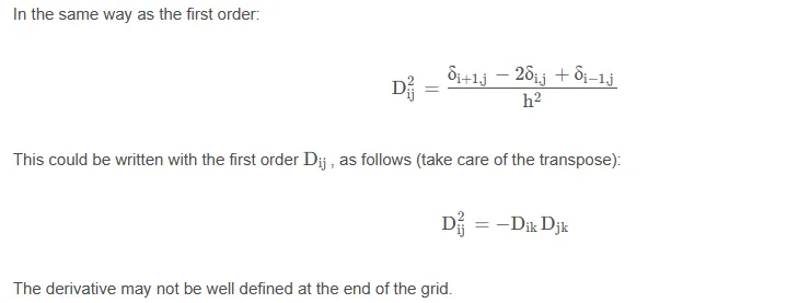
D2=D.dot(-D.T)
D2[-1,-1]=D2[0,0]
2.2 Non-interacting electrons
This is the Hamiltonian of non-interacting free particles in a box given by the size of grid:

eig_non, psi_non=np.linalg.eigh(-D2/2)
plot (energies are shown in the label)
for i in range(3):
    plt.plot(x,psi_non[:,i], label=f"{eig_non[i]:.4f}")
    plt.legend(loc=1)
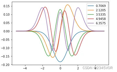
2.3 Harmonic oscillator

X=np.diagflat(x*x)
and solve the KS.
eig_harm, psi_harm = np.linalg.eigh(-D2/2+X)
plot
for i in range(5):
    plt.plot(x,psi_harm[:,i], label=f"{eig_harm[i]:.4f}")
    plt.legend(loc=1)
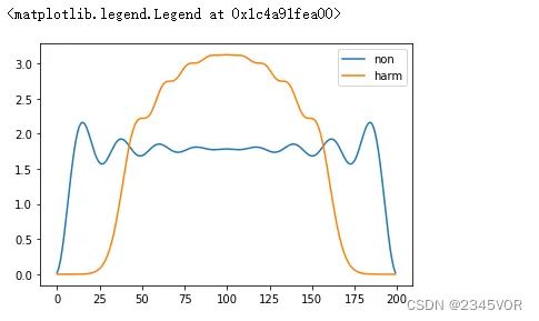
2.4 Density
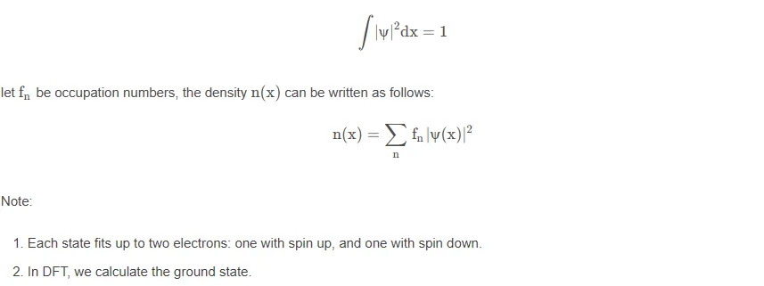
We will want to include the Coulomb or Hatree interacion as well as LDA exchange
Both of which are density functinals
So we need to calculate the electron density
# integral
def integral(x,y,axis=0):
    dx=x[1]-x[0]
    return np.sum(y*dx, axis=axis)
number of electrons
num_electron=17
density
def get_nx(num_electron, psi, x):
    # normalization
    I=integral(x,psi**2,axis=0)
    normed_psi=psi/np.sqrt(I)[None, :]
    # occupation num
    fn=[2 for _ in range(num_electron//2)]
    if num_electron % 2:
        fn.append(1)
    # density
    res=np.zeros_like(normed_psi[:,0])
    for ne, psi  in zip(fn,normed_psi.T):
        res += ne*(psi**2)
    return res
plot
plt.plot(get_nx(num_electron,psi_non, x), label="non")
plt.plot(get_nx(num_electron,psi_harm, x), label="harm")
plt.legend(loc=1)
2.5 Exchange energy
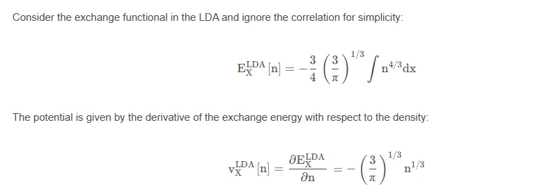
def get_exchange(nx,x):
    energy=-3./4.*(3./np.pi)**(1./3.)*integral(x,nx**(4./3.))
    potential=-(3./np.pi)**(1./3.)*nx**(1./3.)
    return energy, potential
2.6 coulomb potential
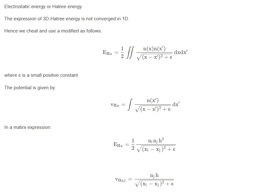
def get_hatree(nx,x, eps=1e-1):
    h=x[1]-x[0]
    energy=np.sum(nx[None,:]*nx[:,None]*h**2/np.sqrt((x[None,:]-x[:,None])**2+eps)/2)
    potential=np.sum(nx[None,:]*h/np.sqrt((x[None,:]-x[:,None])**2+eps),axis=-1)
    return energy, potential
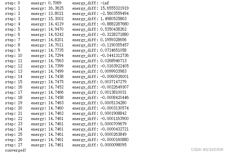
2.7 Solve the KS equation:Self-consistency loop
initialize the density (you can take an arbitrary constant)
Calculate the Exchange and Hatree potentials
Calculate the Hamiltonian
Calculate the wavefunctions and eigen values
If not converged, calculate the density and back to 1.
def print_log(i,log):
    print(f"step: {i:<5} energy: {log['energy'][-1]:<10.4f} energy_diff: {log['energy_diff'][-1]:.10f}")
max_iter=1000
energy_tolerance=1e-5
log={"energy":[float("inf")], "energy_diff":[float("inf")]}
nx=np.zeros(n_grid)
for i in range(max_iter):
    ex_energy, ex_potential=get_exchange(nx,x)
    ha_energy, ha_potential=get_hatree(nx,x)
    # Hamiltonian
    H=-D2/2+np.diagflat(ex_potential+ha_potential+x*x)
    energy, psi= np.linalg.eigh(H)
    # log
    log["energy"].append(energy[0])
    energy_diff=energy[0]-log["energy"][-2]
    log["energy_diff"].append(energy_diff)
    print_log(i,log)
    # convergence
    if abs(energy_diff) < energy_tolerance:
        print("converged!")
        break
    # update density
    nx=get_nx(num_electron,psi,x)
else:
    print("not converged")
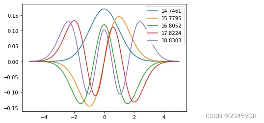
plot
for i in range(5):
    plt.plot(x,psi[:,i], label=f"{energy[i]:.4f}")
    plt.legend(loc=1)
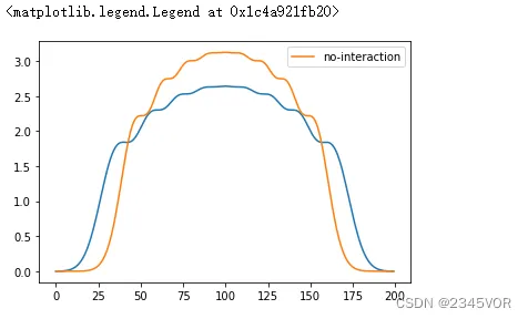
compare the density to free particles
plt.plot(nx)
plt.plot(get_nx(num_electron,psi_harm,x), label="no-interaction")
plt.legend()