How to Configure the Gradient Boosting Algorithm

Gradient boosting is one of the most powerful techniques for applied machine learning and as such is quickly becoming one of the most popular.

But how do you configure gradient boosting on your problem?

In this post you will discover how you can configure gradient boosting on your machine learning problem by looking at configurations reported in books, papers and as a result of competitions.

After reading this post, you will know:

• How to configure gradient boosting according to the original sources.
• Ideas for configuring the algorithm from defaults and suggestions in standard implementations.
• Rules of thumb for configuring gradient boosting and XGBoost from a top Kaggle competitors.

Let’s get started.

How to Configure the Gradient Boosting Algorithm
Photo by Chris Sorge, some rights reserved.

The Algorithm that is Winning Competitions
...XGBoost for fast gradient boosting

XGBoost is the high performance implementation of gradient boosting that you can now access directly in Python. 

Your PDF Download and Email Course.

FREE 7-Day Mini-Course on 
XGBoost With Python

  Download your PDF containing all 7 lessons.

Daily lesson via email with tips and tricks.

How to Configure Gradient Boosting Machines

In the 1999 paper “Greedy Function Approximation: A Gradient Boosting Machine“, Jerome Friedman comments on the trade-off between the number of trees (M) and the learning rate (v):

The v-M trade-off is clearly evident; smaller values of v give rise to larger optimal M-values. They also provide higher accuracy, with a diminishing return for v < 0.125. The misclassification error rate is very flat for M > 200, so that optimal M-values for it are unstable. …  the qualitative nature of these results is fairly universal.

He suggests to first set a large value for the number of trees, then tune the shrinkage parameter to achieve the best results. Studies in the paper preferred a shrinkage value of 0.1, a number of trees in the range 100 to 500 and the number of terminal nodes in a tree between 2 and 8.

In the 1999 paper “Stochastic Gradient Boosting“, Friedman reiterated the preference for the shrinkage parameter:

The “shrinkage” parameter 0 < v < 1 controls the learning rate of the procedure. Empirically …, it was found that small values (v <= 0.1) lead to much better generalization error.

In the paper, Friedman introduces and empirically investigates stochastic gradient boosting (row-based sub-sampling). He finds that almost all subsampling percentages are better than so-called deterministic boosting and perhaps 30%-to-50% is a good value to choose on some problems and 50%-to-80% on others.

… the best value of the sampling fraction … is approximately 40% (f=0.4) … However, sampling only 30% or even 20% of the data at each iteration gives considerable improvement over no sampling at all, with a corresponding computational speed-up by factors of 3 and 5 respectively.

He also studied the effect of the number of terminal nodes in  trees finding values like 3 and 6 better than larger values like 11, 21 and 41.

In both cases the optimal tree size as averaged over 100 targets is L = 6. Increasing the capacity of the base learner by using larger trees degrades performance through “over-fitting”.

In his talk titled “Gradient Boosting Machine Learning” at H2O, Trevor Hastie made the comment that in general gradient boosting performs better than random forest, which in turn performs better than individual decision trees.

Gradient Boosting > Random Forest > Bagging > Single Trees

Chapter 10 titled “Boosting and Additive Trees” of the book “The Elements of Statistical Learning: Data Mining, Inference, and Prediction” is dedicated to boosting. In it they provide both heuristics for configuring gradient boosting as well as some empirical studies.

They comment that a good value the number of nodes in the tree (J) is about 6, with generally good values in the range of 4-to-8.

Although in many applications J = 2 will be insufficient, it is unlikely that J > 10 will be required. Experience so far indicates that 4 <= J <= 8 works well in the context of boosting, with results being fairly insensitive to particular choices in this range.

They suggest monitoring the performance on a validation dataset in order to calibrate the number of trees and to use an early stopping procedure once performance on the validation dataset begins to degrade.

As in Friedman’s first gradient boosting paper, they comment on the trade-off between the number of trees (M) and the learning rate (v) and recommend a small value for the learning rate < 0.1.

Smaller values of v lead to larger values of M for the same training risk, so that there is a tradeoff between them. … In fact, the best strategy appears to be to set v to be very small (v < 0.1) and then choose M by early stopping.

Also, as in Friedman’s stochastic gradient boosting paper, they recommend a subsampling percentage (n) without replacement with a value of about 50%.

A typical value for n can be 1/2, although for large N, n can be substantially smaller than 1/2.

Configuration of Gradient Boosting in R

The gradient boosting algorithm is implemented in R as the gbm package.

Reviewing the package documentation, the gbm() function specifies sensible defaults:

• n.trees = 100 (number of trees).
• interaction.depth = 1 (number of leaves).
• n.minobsinnode = 10 (minimum number of samples in tree terminal nodes).
• shrinkage = 0.001 (learning rate).

It is interesting to note that a smaller shrinkage factor is used and that stumps are the default. The small shrinkage is explained by Ridgeway next.

In the vignette for using the gbm package in R titled “Generalized Boosted Models: A guide to the gbm package“, Greg Ridgeway provides some usage heuristics. He suggest firs setting the learning rate (lambda) to as small as possible then tuning the number of trees (iterations or T) using cross validation.

In practice I set lambda to be as small as possible and then select T by cross-validation. Performance is best when lambda is as small as possible performance with decreasing marginal utility for smaller and smaller lambda.

He comments on his rationale for setting the default shrinkage to the small value of 0.001 rather than 0.1.

It is important to know that smaller values of shrinkage (almost) always give improved predictive performance. That is, setting shrinkage=0.001 will almost certainly result in a model with better out-of-sample predictive performance than setting shrinkage=0.01. …  The model with shrinkage=0.001 will likely require ten times as many iterations as the model with shrinkage=0.01

Ridgeway also uses quite large numbers of trees (called iterations here), thousands rather than hundreds

I usually aim for 3,000 to 10,000 iterations with shrinkage rates between 0.01 and 0.001.

Configuration of Gradient Boosting in scikit-learn

The Python library provides an implementation of gradient boosting for classification called the GradientBoostingClassifier class and regression called the GradientBoostingRegressor class.

It is useful to review the default configuration for the algorithm in this library.

There are many parameters, but below are a few key defaults.

• learning_rate=0.1 (shrinkage).
• n_estimators=100 (number of trees).
• max_depth=3.
• min_samples_split=2.
• min_samples_leaf=1.
• subsample=1.0.

It is interesting to note that the default shrinkage does match Friedman and that the tree depth is not set to stumps like the R package. A tree depth of 3 (if the created tree was symmetrical) will have 8 leaf nodes, matching the upper bound of the preferred number of terminal nodes in Friedman’s studies (alternately max_leaf_nodes can be set).

In the scikit-learn user guide under the section titled “Gradient Tree Boosting” the authors comment that setting the maximum leaf nodes has a similar effect to setting the max depth to one minus the maximum leaf nodes, but results in worse performance.

We found that max_leaf_nodes=k gives comparable results to max_depth=k-1 but is significantly faster to train at the expense of a slightly higher training error.

In a small study demonstrating regularization methods for gradient boosting titled “Gradient Boosting regularization“, the results show the benefit of using both shrinkage and sub-sampling.

Configuration of Gradient Boosting in XGBoost

The XGBoost library is dedicated to the gradient boosting algorithm.

It too specifies default parameters that are interesting to note, firstly the XGBoost Parameters page:

• eta=0.3 (shrinkage or learning rate).
• max_depth=6.
• subsample=1.

This shows a higher learning rate and a larger max depth than we see in most studies and other libraries. Similarly, we can summarize the default parameters for XGBoost in the Python API reference.

• max_depth=3.
• learning_rate=0.1.
• n_estimators=100.
• subsample=1.

These defaults are generally more in-line with scikit-learn defaults and recommendations from the papers.

In a talk to TechEd Europe titled “xgboost: An R package for Fast and Accurate Gradient Boosting“, when asked how to configure XGBoost, Tong He suggested the three most important parameters to tune are:

• Number of trees.
• Tree depth.
• Step Size (learning rate).

He also provide a terse configuration strategy for new problems:

1. Run the default configuration (and presumably review learning curves?).
2. If the system is overlearning, slow the learning down (using shrinkage?).
3. If the system is underlearning, speed the learning up to be more aggressive (using shrinkage?).

In Owen Zhang’s talk to the NYC Data Science Academy in 2015 titled “Winning Data Science Competitions“, he provides some general tips for configuring gradient boost with XGBoost. Owen is a heavy user of gradient boosting.

My confession: I (over)use GBM. When in doubt, use GBM.

He provides some tips for configuring gradient boosting:

• learning rate + number of trees: Target 500-to-1000 trees and tune learning rate.
• number of samples in leaf: the number of observations needed to get a good mean estimate.
• interaction depth: 10+.

In an updated slide deck for the same talk, he gives a summary of common parameters he uses for XGBoost:

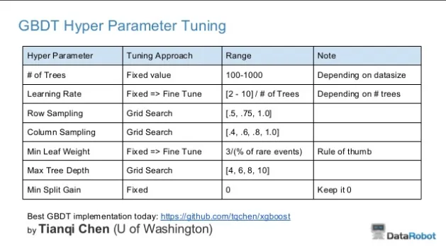
Owen Zhang Table of Suggestions for Hyperparameter Tuning of XGBoost

We can see a few interesting things in this table.

• Simplified the relationship of learning rate and the number of trees as an approximate ratio: learning rate = [2-10]/trees.
• Explores values for both row and column sampling for stochastic gradient boosting.
• Explores close to the same range for max depth as reported by Friedman (4-10).
• Tunes minimum leaf weight as an approximate ratio of 3 over the percentage of the number of rare events.

In a similar talk by Owen at ODSC Boston 2015 titled “Open Source Tools and Data Science Competitions“, he again summarized common parameters he uses:

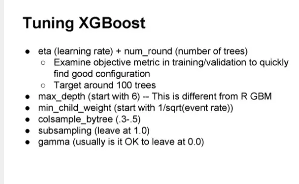
Owen Zhang Suggestions for Tuning XGBoost

We can see some minor differences that may be relevant.

• Target 100 rather than 1000 trees and tune learning rate.
• Min child weight as 1 over the square root of the event rate.
• No sub sampling of rows.

Finally, Abhishek Thakur, in his post titled “Approaching (Almost) Any Machine Learning Problem” provided a similar table listing out key XGBoost parameters and suggestions for tuning.

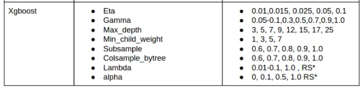
Abhishek Thakur Suggestions for Tuning XGBoost

The spreads do cover the general defaults suggested above and more.

It is interesting to note that Abhishek does provides some suggestions for tuning the alpha and beta model penalization terms as well as row sampling.

Want to Systematically Learn How To Use XGBoost?

You can develop and evaluate XGBoost models in just a few lines of Python code. You need:

>> XGBoost With Python

Take the next step with 15 self-study tutorial lessons.

Covers building large models on Amazon Web Services, feature importance, tree visualization, hyperparameter tuning, and much more...

Ideal for machine learning practitioners already familiar with the Python ecosystem.

Bring XGBoost To Your Machine Learning Projects

Summary

In this post you got insight into how to configure gradient boosting for your own machine learning problems.

Specifically you learned:

• About the trade-off in the number of trees and the shrinkage and good defaults for sub-sampling.
• Different ideas on limiting tree size and good defaults for tree depth and the number of terminal nodes.
• Grid search strategies used by a top Kaggle competition winner.

Do you have any questions about configuring gradient boosting or about this post? Ask your questions in the comments.