多项式拟合实例
导入必要的模块
import numpy as np
import pandas as pd
import matplotlib.pyplot as plt
from sklearn.preprocessing import StandardScaler
from sklearn.preprocessing import PolynomialFeatures
from sklearn.linear_model import LinearRegression, Ridge
from sklearn.metrics import mean_squared_error
生成数据
生成100个训练样本
# 设置随机种子
np.random.seed(34)

sample_num = 100

# 从-5到5中随机抽取100个浮点数
x_train = np.random.uniform(-5, 5, size=sample_num)

# 将x从shape为(sample_num,)变为(sample_num,1)
X_train = x_train.reshape(-1,1)

# 生成y值的实际函数
y_train_real = 0.5 * x_train ** 3 + x_train ** 2 + 2 * x_train + 1

# 生成误差值
err_train = np.random.normal(0, 5, size=sample_num)

# 真实y值加上误差值,得到样本的y值
y_train = y_train_real + err_train

# 画出样本的散点图
plt.scatter(x_train, y_train, marker='o', color='g', label='train dataset')

# 画出实际函数曲线
plt.plot(np.sort(x_train), y_train_real[np.argsort(x_train)], color='b', label='real curve')
plt.legend()
plt.xlabel('x')
plt.ylabel('y')
plt.show()

生成测试集
# 设置随机种子
np.random.seed(12)

sample_num = 100

# 从-5到5中随机抽取100个浮点数
x_test = np.random.uniform(-5, 5, size=sample_num)

# 将x从shape为(sample_num,)变为(sample_num,1)
X_test = x_test.reshape(-1,1)

# 生成y值的实际函数
y_test_real = 0.5 * x_test ** 3 + x_test ** 2 + 2 * x_test + 1

# 生成误差值
err_test = np.random.normal(0, 5, size=sample_num)

# 真实y值加上误差值,得到样本的y值
y_test = y_test_real + err_test

# 画出样本的散点图
plt.scatter(x_test, y_test, marker='o', color='c', label='test dataset')
plt.legend()
plt.xlabel('x')
plt.ylabel('y')
plt.show()

问题:加入我们不知道生成样本的函数,如何用线性回归模型拟合这些样本?
多项式模型拟合
1阶线性模型拟合
# 线性回归模型训练
reg1 = LinearRegression()
reg1.fit(X_train, y_train)

# 模型预测
y_train_pred1 = reg1.predict(X_train)

# 画出样本的散点图
plt.scatter(x_train, y_train, marker='o', color='g', label='train dataset')

# 画出实际函数曲线
plt.plot(np.sort(x_train), y_train_real[np.argsort(x_train)], color='b', label='real curve')

# 画出预测函数曲线
plt.plot(np.sort(x_train), y_train_pred1[np.argsort(x_train)], color='r', label='prediction curve')
plt.legend()
plt.xlabel('x')
plt.ylabel('y')
plt.show()

直线太过简单,不能很好地描述数据的变化关系。
3阶多项式模型拟合
使用到的api:
创建多项式特征sklearn.preprocessing.PolynomialFeatures
用到的参数:
- degree:设置多项式特征的阶数,默认2。
- include_bias:是否包括偏置项,默认True。
使用fit_transform函数对数据做处理。
特征标准化sklearn.preprocessing.StandardScaler(减去均值除再除以标准差)
使用fit_transform函数对数据做处理。
# 生成多项式数据
poly = PolynomialFeatures(degree=3, include_bias=False)
X_train_poly = poly.fit_transform(X_train)

# 数据标准化(减均值除标准差)
scaler  = StandardScaler()
X_train_poly_scaled = scaler.fit_transform(X_train_poly)

# 线性回归模型训练
reg3 = LinearRegression()
reg3.fit(X_train_poly_scaled, y_train)

# 模型预测
y_train_pred3 = reg3.predict(X_train_poly_scaled)

# 画出样本的散点图
plt.scatter(x_train, y_train, marker='o', color='g', label='train dataset')

# 画出实际函数曲线
# plt.plot(np.sort(x_train), y_train_real[np.argsort(x_train)], color='b', label='real curve')

# 画出预测函数曲线
plt.plot(np.sort(x_train), y_train_pred3[np.argsort(x_train)], color='r', label='prediction curve')
plt.legend()
plt.xlabel('x')
plt.ylabel('y')
plt.show()

曲线拟合得非常不错。
10阶多项式模型拟合
# 生成多项式数据
poly = PolynomialFeatures(degree=10, include_bias=False)
X_train_poly = poly.fit_transform(X_train)

# 数据标准化(减均值除标准差)
scaler  = StandardScaler()
X_train_poly_scaled = scaler.fit_transform(X_train_poly)

# 线性回归模型训练
reg10 = LinearRegression()
reg10.fit(X_train_poly_scaled, y_train)

# 模型预测
y_train_pred10 = reg10.predict(X_train_poly_scaled)

# 画出样本的散点图
plt.scatter(x_train, y_train, marker='o', color='g', label='train dataset')

# 画出实际函数曲线
plt.plot(np.sort(x_train), y_train_real[np.argsort(x_train)], color='b', label='real curve')

# 画出预测函数曲线
plt.plot(np.sort(x_train), y_train_pred10[np.argsort(x_train)], color='r', label='prediction curve')
plt.legend()
plt.xlabel('x')
plt.ylabel('y')
plt.show()

曲线拟合得也还可以。
30阶多项式模型拟合
# 生成多项式数据
poly = PolynomialFeatures(degree=30, include_bias=False)
X_train_poly = poly.fit_transform(X_train)

# 数据标准化(减均值除标准差)
scaler  = StandardScaler()
X_train_poly_scaled = scaler.fit_transform(X_train_poly)

# 线性回归模型训练
reg30 = LinearRegression()
reg30.fit(X_train_poly_scaled, y_train)

# 模型预测
y_train_pred30 = reg30.predict(X_train_poly_scaled)

# 画出样本的散点图
plt.scatter(x_train, y_train, marker='o', color='g', label='train dataset')

# 画出实际函数曲线
# plt.plot(np.sort(x_train), y_train_real[np.argsort(x_train)], color='b', label='real curve')

# 画出预测函数曲线
plt.plot(np.sort(x_train), y_train_pred30[np.argsort(x_train)], color='r', label='prediction curve')
plt.legend()
plt.xlabel('x')
plt.ylabel('y')
plt.show()

曲线变得弯曲而复杂,把训练样本点的噪声变化也学习到了。
指标对比
# 计算MSE
mse1 = mean_squared_error(y_train_pred1, y_train)
mse3 = mean_squared_error(y_train_pred3, y_train)
mse10 = mean_squared_error(y_train_pred10, y_train)
mse30 = mean_squared_error(y_train_pred30, y_train)

# 打印结果
print('MSE:')
print('1 order polynomial: {:.2f}'.format(mse1))
print('3 order polynomial: {:.2f}'.format(mse3))
print('10 order polynomial: {:.2f}'.format(mse10))
print('30 order polynomial: {:.2f}'.format(mse30))
MSE:
1 order polynomial: 149.92
3 order polynomial: 24.32
10 order polynomial: 23.64
30 order polynomial: 15.05
训练集mse指标从好到坏的模型是:30阶多项式、10阶多项式、3阶多项式、1阶多项式。
测试集检验
1阶线性模型预测
# 模型预测
y_test_pred1 = reg1.predict(X_test)

# 画出样本的散点图
plt.scatter(x_test, y_test, marker='o', color='c', label='test dataset')

# 画出预测函数曲线
plt.plot(np.sort(x_test), y_test_pred1[np.argsort(x_test)], color='r', label='1 order')
plt.legend()
plt.xlabel('x')
plt.ylabel('y')
plt.show()

3阶多项式模型预测
# 生成多项式数据
poly = PolynomialFeatures(degree=3, include_bias=False)
X_test_poly = poly.fit_transform(X_test)

# 数据标准化(减均值除标准差)
scaler  = StandardScaler()
X_test_poly_scaled = scaler.fit_transform(X_test_poly)

# 模型预测
y_test_pred3 = reg3.predict(X_test_poly_scaled)

# 画出样本的散点图
plt.scatter(x_test, y_test, marker='o', color='c', label='test dataset')

# 画出预测函数曲线
plt.plot(np.sort(x_test), y_test_pred3[np.argsort(x_test)], color='r', label='3 order')
plt.legend()
plt.xlabel('x')
plt.ylabel('y')
plt.show()

10阶多项式模型预测
# 生成多项式数据
poly = PolynomialFeatures(degree=10, include_bias=False)
X_test_poly = poly.fit_transform(X_test)

# 数据标准化(减均值除标准差)
scaler  = StandardScaler()
X_test_poly_scaled = scaler.fit_transform(X_test_poly)

# 模型预测
y_test_pred10 = reg10.predict(X_test_poly_scaled)

# 画出样本的散点图
plt.scatter(x_test, y_test, marker='o', color='c', label='test dataset')

# 画出预测函数曲线
plt.plot(np.sort(x_test), y_test_pred10[np.argsort(x_test)], color='r', label='10 order')
plt.legend()
plt.xlabel('x')
plt.ylabel('y')
plt.show()

30阶多项式模型预测
# 生成多项式数据
poly = PolynomialFeatures(degree=30, include_bias=False)
X_test_poly = poly.fit_transform(X_test)

# 数据标准化(减均值除标准差)
scaler  = StandardScaler()
X_test_poly_scaled = scaler.fit_transform(X_test_poly)

# 模型预测
y_test_pred30 = reg30.predict(X_test_poly_scaled)

# 画出样本的散点图
plt.scatter(x_test, y_test, marker='o', color='c', label='test dataset')

# 画出预测函数曲线
plt.plot(np.sort(x_test), y_test_pred30[np.argsort(x_test)], color='r', label='30 order')
plt.legend()
plt.xlabel('x')
plt.ylabel('y')
plt.show()

指标对比
# 计算MSE
mse1 = mean_squared_error(y_test_pred1, y_test)
mse3 = mean_squared_error(y_test_pred3, y_test)
mse10 = mean_squared_error(y_test_pred10, y_test)
mse30 = mean_squared_error(y_test_pred30, y_test)

# 打印结果
print('MSE:')
print('1 order polynomial: {:.2f}'.format(mse1))
print('3 order polynomial: {:.2f}'.format(mse3))
print('10 order polynomial: {:.2f}'.format(mse10))
print('30 order polynomial: {:.2f}'.format(mse30))
MSE:
1 order polynomial: 191.05
3 order polynomial: 39.71
10 order polynomial: 41.00
30 order polynomial: 85.45
测试集mse指标从好到坏的模型是:3阶多项式、10阶多项式、30阶多项式、1阶多项式。
欠拟合和过拟合
欠拟合(Underfitting):选择的模型过于简单,以致于模型对训练集和未知数据的预测都很差的现象。
过拟合(Overfitting):选择的模型过于复杂(所包含的参数过多),以致于模型对训练集的预测很好,但对未知数据预测很差的现象(泛化能力差)。
过拟合常见解决方法
增加训练样本数目
生成200个训练样本
# 设置随机种子
np.random.seed(34)

sample_num = 200

# 从-10到10中随机抽取200个浮点数
x_train = np.random.uniform(-10, 10, size=sample_num)

# 将x从shape为(sample_num,)变为(sample_num,1)
X_train = x_train.reshape(-1,1)

# 生成y值的实际函数
y_train_real = 0.5 * x_train ** 3 + x_train ** 2 + 2 * x_train + 1

# 生成误差值
err_train = np.random.normal(0, 5, size=sample_num)

# 真实y值加上误差值,得到样本的y值
y_train = y_train_real + err_train

# 画出样本的散点图
plt.scatter(x_train, y_train, marker='o', color='g')

# 画出实际函数曲线
plt.plot(np.sort(x_train), y_train_real[np.argsort(x_train)], color='b', label='real curve')
plt.legend()
plt.xlabel('x')
plt.ylabel('y')
plt.show()

30阶多项式模型训练
# 生成多项式数据
poly = PolynomialFeatures(degree=30, include_bias=False)
X_train_poly = poly.fit_transform(X_train)

# 数据标准化(减均值除标准差)
scaler  = StandardScaler()
X_train_poly_scaled = scaler.fit_transform(X_train_poly)

# 线性回归模型训练
reg30 = LinearRegression()
reg30.fit(X_train_poly_scaled, y_train)

# 模型预测
y_train_pred30 = reg30.predict(X_train_poly_scaled)

# 画出样本的散点图
plt.scatter(x_train, y_train, marker='o', color='g')

# 画出实际函数曲线
plt.plot(np.sort(x_train), y_train_real[np.argsort(x_train)], color='b', label='real curve')

# 画出预测函数曲线
plt.plot(np.sort(x_train), y_train_pred30[np.argsort(x_train)], color='r', label='prediction curve')
plt.legend()
plt.xlabel('x')
plt.ylabel('y')
plt.show()

# 计算MSE
mse = mean_squared_error(y_train_pred30, y_train)
print('MSE: {}'.format(mse))

MSE: 24.924693781595153
30阶多项式模型预测
# 生成多项式数据
poly = PolynomialFeatures(degree=30, include_bias=False)
X_test_poly = poly.fit_transform(X_test)

# 数据标准化(减均值除标准差)
scaler  = StandardScaler()
X_test_poly_scaled = scaler.fit_transform(X_test_poly)

# 模型预测
y_test_pred30 = reg30.predict(X_test_poly_scaled)

# 画出样本的散点图
plt.scatter(x_test, y_test, marker='o', color='c', label='test dataset')

# 画出预测函数曲线
plt.plot(np.sort(x_test), y_test_pred30[np.argsort(x_test)], color='r', label='30 order')
plt.legend()
plt.xlabel('x')
plt.ylabel('y')
plt.show()

计算MSE
mse30 = mean_squared_error(y_test_pred30, y_test)

# 打印结果
print('MSE:')
print('30 order polynomial: {:.2f}'.format(mse30))
MSE:
30 order polynomial: 32.32
在目标函数中增加正则项
查看回归系数
将结果转换为pd.DataFrame表格形式
coef1 = pd.DataFrame(reg1.coef_, index=['w1'], columns=['coef'])
coef3 = pd.DataFrame(reg3.coef_, index=['w1', 'w2', 'w3'], columns=['coef'])
coef10 = pd.DataFrame(reg10.coef_, index=['w'+str(i) for i in range(1,11)], columns=['coef'])
coef30 = pd.DataFrame(reg30.coef_, index=['w'+str(i) for i in range(1,31)], columns=['coef'])
1阶多项式模型参数
coef1
coef
w1
9.900252
3阶多项式模型参数
coef3
coef
w1
7.789175
w2
7.000036
w3
25.295452
10阶多项式模型参数
coef10
coef
w1
7.998547
w2
4.203915
w3
20.728305
w4
15.694967
w5
10.679321
w6
-53.302415
w7
-5.051154
w8
72.956004
w9
-1.464603
w10
-32.583643
30阶多项式模型参数
coef30
coef
w1
1.274825e+01
w2
-1.515071e+02
w3
-2.784062e+02
w4
9.881947e+03
w5
8.313355e+03
w6
-2.294226e+05
w7
-1.443295e+05
w8
2.805398e+06
w9
1.540533e+06
w10
-2.094909e+07
w11
-1.036432e+07
w12
1.035820e+08
w13
4.594186e+07
w14
-3.558672e+08
w15
-1.390464e+08
w16
8.741809e+08
w17
2.938075e+08
w18
-1.558118e+09
w19
-4.373421e+08
w20
2.020758e+09
w21
4.563577e+08
w22
-1.888828e+09
w23
-3.264643e+08
w24
1.240156e+09
w25
1.523610e+08
w26
-5.429771e+08
w27
-4.173929e+07
w28
1.424089e+08
w29
5.084136e+06
w30
-1.693219e+07
模型太复杂(阶数过多),发生过拟合时,系数绝对值往往会很大,输入x的很小变化都可能带来输出y较大的变化,导致函数变化剧烈。
训练Ridge回归(加L2正则)
使用到的api:
加L2正则的线性回归sklearn.linear_model.Ridge
用到的参数:
- alpha:惩罚项,默认1.0。
# 生成多项式数据
poly = PolynomialFeatures(degree=30, include_bias=False)
X_train_poly = poly.fit_transform(X_train)

# 数据标准化(减均值除标准差)
scaler  = StandardScaler()
X_train_poly_scaled = scaler.fit_transform(X_train_poly)

# 线性回归模型训练
ridge30 = Ridge(alpha=1e-5)
ridge30.fit(X_train_poly_scaled, y_train)

# 模型预测
y_train_pred30 = ridge30.predict(X_train_poly_scaled)

# 画出样本的散点图
plt.scatter(x_train, y_train, marker='o', color='g')

# 画出实际函数曲线
plt.plot(np.sort(x_train), y_train_real[np.argsort(x_train)], color='b', label='real curve')

# 画出预测函数曲线
plt.plot(np.sort(x_train), y_train_pred30[np.argsort(x_train)], color='r', label='prediction curve')
plt.legend()
plt.xlabel('x')
plt.ylabel('y')
plt.show()

# 计算MSE
mse = mean_squared_error(y_train_pred30, y_train)
print('MSE: {}'.format(mse))

MSE: 22.402223562860904
查看加正则后的回归系数
将结果转换为pd.DataFrame表格形式
coef30 = pd.DataFrame(ridge30.coef_, index=['w'+str(i) for i in range(1,31)], columns=['coef'])
coef30
coef
w1
10.011475
w2
3.557561
w3
-4.055929
w4
7.173610
w5
100.444037
w6
26.619616
w7
-75.014554
w8
-90.566477
w9
-182.926719
w10
-16.985565
w11
172.986261
w12
101.786157
w13
257.743919
w14
114.148735
w15
14.865358
w16
11.446063
w17
-256.410160
w18
-117.329198
w19
-313.210519
w20
-169.444870
w21
-113.923505
w22
-95.081604
w23
205.527433
w24
73.135599
w25
413.318846
w26
222.862257
w27
261.405747
w28
183.223254
w29
-458.772050
w30
-248.055649
模型检验
# 生成多项式数据
poly = PolynomialFeatures(degree=30, include_bias=False)
X_test_poly = poly.fit_transform(X_test)

# 数据标准化(减均值除标准差)
scaler  = StandardScaler()
X_test_poly_scaled = scaler.fit_transform(X_test_poly)

# 模型预测
y_test_pred30 = ridge30.predict(X_test_poly_scaled)

# 画出样本的散点图
plt.scatter(x_test, y_test, marker='o', color='c', label='test dataset')

# 画出预测函数曲线
plt.plot(np.sort(x_test), y_test_pred30[np.argsort(x_test)], color='r', label='30 order')
plt.legend()
plt.xlabel('x')
plt.ylabel('y')
plt.show()

计算MSE
mse30 = mean_squared_error(y_test_pred30, y_test)

# 打印结果
print('MSE:')
print('30 order polynomial: {:.2f}'.format(mse30))
MSE:
30 order polynomial: 28.80