目录
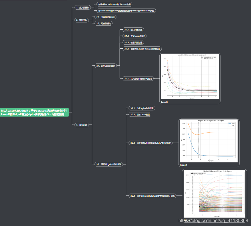
基于datasets糖尿病数据集利用LassoR和RidgeR算法(alpha调参)进行(9→1)回归预测
相关文章
ML之LassoR&RidgeR:基于datasets糖尿病数据集利用LassoR和RidgeR算法(alpha调参)进行(9→1)回归预测
ML之LassoR&RidgeR:基于datasets糖尿病数据集利用LassoR和RidgeR算法(alpha调参)进行(9→1)回归预测实现
基于datasets糖尿病数据集利用LassoR和RidgeR算法(alpha调参)进行(9→1)回归预测
设计思路
输出结果
1. .. _diabetes_dataset:
2.
3. Diabetes dataset
4. ----------------
5.
6. Ten baseline variables, age, sex, body mass index, average blood
7. pressure, and six blood serum measurements were obtained for each of n =
8. 442 diabetes patients, as well as the response of interest, a
9. quantitative measure of disease progression one year after baseline.
10.
11. **Data Set Characteristics:**
12.
13.   :Number of Instances: 442
14.
15.   :Number of Attributes: First 10 columns are numeric predictive values
16.
17.   :Target: Column 11 is a quantitative measure of disease progression one year after baseline
18.
19.   :Attribute Information:
20.       - age     age in years
21.       - sex
22.       - bmi     body mass index
23.       - bp      average blood pressure
24.       - s1      tc, T-Cells (a type of white blood cells)
25.       - s2      ldl, low-density lipoproteins
26.       - s3      hdl, high-density lipoproteins
27.       - s4      tch, thyroid stimulating hormone
28.       - s5      ltg, lamotrigine
29.       - s6      glu, blood sugar level
30.
31. Note: Each of these 10 feature variables have been mean centered and scaled by the standard deviation times `n_samples` (i.e. the sum of squares of each column totals 1).
32.
33. Source URL:
34. https://www4.stat.ncsu.edu/~boos/var.select/diabetes.html
35.
36. For more information see:
37. Bradley Efron, Trevor Hastie, Iain Johnstone and Robert Tibshirani (2004) "Least Angle Regression," Annals of Statistics (with discussion), 407-499.
38. (https://web.stanford.edu/~hastie/Papers/LARS/LeastAngle_2002.pdf)
39.         age       sex       bmi        bp  ...        s4        s5        s6  target
40. 0  0.038076  0.050680  0.061696  0.021872  ... -0.002592  0.019908 -0.017646   151.0
41. 1 -0.001882 -0.044642 -0.051474 -0.026328  ... -0.039493 -0.068330 -0.092204    75.0
42. 2  0.085299  0.050680  0.044451 -0.005671  ... -0.002592  0.002864 -0.025930   141.0
43. 3 -0.089063 -0.044642 -0.011595 -0.036656  ...  0.034309  0.022692 -0.009362   206.0
44. 4  0.005383 -0.044642 -0.036385  0.021872  ... -0.002592 -0.031991 -0.046641   135.0
45.
46. [5 rows x 11 columns]
47. alphas:  50 [1.00000000e-03 1.16779862e-03 1.36375363e-03 1.59258961e-03
48.  1.85982395e-03 2.17189985e-03 2.53634166e-03 2.96193630e-03
49.  3.45894513e-03 4.03935136e-03 4.71714896e-03 5.50868007e-03
50.  6.43302900e-03 7.51248241e-03 8.77306662e-03 1.02451751e-02
51.  1.19643014e-02 1.39718947e-02 1.63163594e-02 1.90542221e-02
52.  2.22514943e-02 2.59852645e-02 3.03455561e-02 3.54374986e-02
53.  4.13838621e-02 4.83280172e-02 5.64373920e-02 6.59075087e-02
54.  7.69666979e-02 8.98816039e-02 1.04963613e-01 1.22576363e-01
55.  1.43144508e-01 1.67163960e-01 1.95213842e-01 2.27970456e-01
56.  2.66223585e-01 3.10895536e-01 3.63063379e-01 4.23984915e-01
57.  4.95129000e-01 5.78210965e-01 6.75233969e-01 7.88537299e-01
58.  9.20852773e-01 1.07537060e+00 1.25581631e+00 1.46654056e+00
59.  1.71262404e+00 2.00000000e+00]
60. {'alpha': 0.07696669794067007}
61. 0.472 (+/-0.177) for {'alpha': 0.0010000000000000002}
62. 0.472 (+/-0.177) for {'alpha': 0.0011677986237376523}
63. 0.472 (+/-0.177) for {'alpha': 0.0013637536256035543}
64. 0.472 (+/-0.177) for {'alpha': 0.0015925896070970653}
65. 0.472 (+/-0.177) for {'alpha': 0.0018598239513468405}
66. 0.472 (+/-0.176) for {'alpha': 0.002171899850777162}
67. 0.472 (+/-0.176) for {'alpha': 0.0025363416566335814}
68. 0.472 (+/-0.176) for {'alpha': 0.002961936295945173}
69. 0.472 (+/-0.176) for {'alpha': 0.0034589451300033745}
70. 0.472 (+/-0.176) for {'alpha': 0.004039351362401994}
71. 0.472 (+/-0.176) for {'alpha': 0.004717148961805858}
72. 0.472 (+/-0.176) for {'alpha': 0.0055086800655623795}
73. 0.472 (+/-0.176) for {'alpha': 0.00643302899917478}
74. 0.472 (+/-0.176) for {'alpha': 0.007512482411700719}
75. 0.471 (+/-0.175) for {'alpha': 0.008773066621237415}
76. 0.471 (+/-0.174) for {'alpha': 0.010245175126239786}
77. 0.471 (+/-0.174) for {'alpha': 0.011964301412374057}
78. 0.472 (+/-0.173) for {'alpha': 0.013971894723352857}
79. 0.472 (+/-0.173) for {'alpha': 0.016316359428938842}
80. 0.473 (+/-0.172) for {'alpha': 0.01905422208552364}
81. 0.473 (+/-0.171) for {'alpha': 0.02225149432786609}
82. 0.474 (+/-0.170) for {'alpha': 0.025985264452188187}
83. 0.474 (+/-0.169) for {'alpha': 0.03034555606472431}
84. 0.475 (+/-0.167) for {'alpha': 0.03543749860893881}
85. 0.476 (+/-0.166) for {'alpha': 0.04138386210422369}
86. 0.477 (+/-0.164) for {'alpha': 0.04832801721026122}
87. 0.477 (+/-0.162) for {'alpha': 0.05643739198611263}
88. 0.478 (+/-0.160) for {'alpha': 0.06590750868872472}
89. 0.478 (+/-0.157) for {'alpha': 0.07696669794067007}
90. 0.477 (+/-0.154) for {'alpha': 0.08988160392874607}
91. 0.476 (+/-0.151) for {'alpha': 0.10496361336732249}
92. 0.475 (+/-0.148) for {'alpha': 0.12257636323289021}
93. 0.472 (+/-0.145) for {'alpha': 0.1431445082861357}
94. 0.469 (+/-0.143) for {'alpha': 0.1671639597721522}
95. 0.466 (+/-0.139) for {'alpha': 0.19521384216045554}
96. 0.462 (+/-0.134) for {'alpha': 0.22797045620951942}
97. 0.455 (+/-0.129) for {'alpha': 0.2662235850143214}
98. 0.447 (+/-0.126) for {'alpha': 0.31089553618622834}
99. 0.441 (+/-0.122) for {'alpha': 0.3630633792844568}
100. 0.434 (+/-0.117) for {'alpha': 0.42398491465793015}
101. 0.425 (+/-0.112) for {'alpha': 0.49512899982305664}
102. 0.412 (+/-0.107) for {'alpha': 0.5782109645659657}
103. 0.395 (+/-0.105) for {'alpha': 0.675233968650155}
104. 0.374 (+/-0.103) for {'alpha': 0.7885372992905638}
105. 0.348 (+/-0.102) for {'alpha': 0.9208527728773261}
106. 0.314 (+/-0.095) for {'alpha': 1.075370600831142}
107. 0.272 (+/-0.089) for {'alpha': 1.2558163076585396}
108. 0.212 (+/-0.084) for {'alpha': 1.466540555750942}
109. 0.129 (+/-0.087) for {'alpha': 1.7126240426614014}
110. 0.018 (+/-0.098) for {'alpha': 2.0}
111. m_log_alphas:  100 [-0.77418297 -0.70440767 -0.63463236 -0.56485706 -0.49508175 -0.42530644
112.  -0.35553114 -0.28575583 -0.21598053 -0.14620522 -0.07642991 -0.00665461
113.   0.0631207   0.132896    0.20267131  0.27244662  0.34222192  0.41199723
114.   0.48177253  0.55154784  0.62132314  0.69109845  0.76087376  0.83064906
115.   0.90042437  0.97019967  1.03997498  1.10975029  1.17952559  1.2493009
116.   1.3190762   1.38885151  1.45862681  1.52840212  1.59817743  1.66795273
117.   1.73772804  1.80750334  1.87727865  1.94705396  2.01682926  2.08660457
118.   2.15637987  2.22615518  2.29593048  2.36570579  2.4354811   2.5052564
119.   2.57503171  2.64480701  2.71458232  2.78435763  2.85413293  2.92390824
120.   2.99368354  3.06345885  3.13323415  3.20300946  3.27278477  3.34256007
121.   3.41233538  3.48211068  3.55188599  3.6216613   3.6914366   3.76121191
122.   3.83098721  3.90076252  3.97053783  4.04031313  4.11008844  4.17986374
123.   4.24963905  4.31941435  4.38918966  4.45896497  4.52874027  4.59851558
124.   4.66829088  4.73806619  4.8078415   4.8776168   4.94739211  5.01716741
125.   5.08694272  5.15671802  5.22649333  5.29626864  5.36604394  5.43581925
126.   5.50559455  5.57536986  5.64514517  5.71492047  5.78469578  5.85447108
127.   5.92424639  5.99402169  6.063797    6.13357231]
128. 交叉验证选择的alpha: 0.06176875494949271
129. (100, 10) (100,)
130. alphas:  50 [1.00000000e-04 1.22398508e-04 1.49813947e-04 1.83370035e-04
131.  2.24442186e-04 2.74713886e-04 3.36245696e-04 4.11559714e-04
132.  5.03742947e-04 6.16573850e-04 7.54677190e-04 9.23713617e-04
133.  1.13061168e-03 1.38385182e-03 1.69381398e-03 2.07320303e-03
134.  2.53756957e-03 3.10594728e-03 3.80163312e-03 4.65314220e-03
135.  5.69537661e-03 6.97105597e-03 8.53246847e-03 1.04436141e-02
136.  1.27828277e-02 1.56459904e-02 1.91504587e-02 2.34398757e-02
137.  2.86900580e-02 3.51162028e-02 4.29817081e-02 5.26089693e-02
138.  6.43925932e-02 7.88155731e-02 9.64690852e-02 1.18076721e-01
139.  1.44524144e-01 1.76895395e-01 2.16517323e-01 2.65013972e-01
140.  3.24373147e-01 3.97027891e-01 4.85956213e-01 5.94803152e-01
141.  7.28030181e-01 8.91098077e-01 1.09069075e+00 1.33498920e+00
142.  1.63400685e+00 2.00000000e+00]
143. m_log_alphas:  50 [ 9.21034037  9.00822838  8.80611639  8.6040044   8.40189241  8.19978042
144.   7.99766843  7.79555644  7.59344445  7.39133245  7.18922046  6.98710847
145.   6.78499648  6.58288449  6.3807725   6.17866051  5.97654852  5.77443653
146.   5.57232454  5.37021255  5.16810055  4.96598856  4.76387657  4.56176458
147.   4.35965259  4.1575406   3.95542861  3.75331662  3.55120463  3.34909264
148.   3.14698065  2.94486866  2.74275666  2.54064467  2.33853268  2.13642069
149.   1.9343087   1.73219671  1.53008472  1.32797273  1.12586074  0.92374875
150.   0.72163676  0.51952476  0.31741277  0.11530078 -0.08681121 -0.2889232
151.  -0.49103519 -0.69314718]
152. 交叉验证选择的alpha: 0.0046531422008170295
核心代码
1. class Ridge Found at: sklearn.linear_model._ridge
2.
3. class Ridge(MultiOutputMixin, RegressorMixin, _BaseRidge):
4. """Linear least squares with l2 regularization.
5.
6.     Minimizes the objective function::
7.
8.     ||y - Xw||^2_2 + alpha * ||w||^2_2
9.
10.     This model solves a regression model where the loss function is
11.     the linear least squares function and regularization is given by
12.     the l2-norm. Also known as Ridge Regression or Tikhonov regularization.
13.     This estimator has built-in support for multi-variate regression
14.     (i.e., when y is a 2d-array of shape (n_samples, n_targets)).
15.
16.     Read more in the :ref:`User Guide <ridge_regression>`.
17.
18.     Parameters
19.     ----------
20.     alpha : {float, ndarray of shape (n_targets,)}, default=1.0
21.     Regularization strength; must be a positive float. Regularization
22.     improves the conditioning of the problem and reduces the variance of
23.     the estimates. Larger values specify stronger regularization.
24.     Alpha corresponds to ``1 / (2C)`` in other linear models such as
25.     :class:`~sklearn.linear_model.LogisticRegression` or
26.     :class:`sklearn.svm.LinearSVC`. If an array is passed, penalties are
27.     assumed to be specific to the targets. Hence they must correspond in
28.     number.
29.
30.     fit_intercept : bool, default=True
31.     Whether to fit the intercept for this model. If set
32.     to false, no intercept will be used in calculations
33.     (i.e. ``X`` and ``y`` are expected to be centered).
34.
35.     normalize : bool, default=False
36.     This parameter is ignored when ``fit_intercept`` is set to False.
37.     If True, the regressors X will be normalized before regression by
38.     subtracting the mean and dividing by the l2-norm.
39.     If you wish to standardize, please use
40.     :class:`sklearn.preprocessing.StandardScaler` before calling ``fit``
41.     on an estimator with ``normalize=False``.
42.
43.     copy_X : bool, default=True
44.     If True, X will be copied; else, it may be overwritten.
45.
46.     max_iter : int, default=None
47.     Maximum number of iterations for conjugate gradient solver.
48.     For 'sparse_cg' and 'lsqr' solvers, the default value is determined
49.     by scipy.sparse.linalg. For 'sag' solver, the default value is 1000.
50.
51.     tol : float, default=1e-3
52.     Precision of the solution.
53.
54.     solver : {'auto', 'svd', 'cholesky', 'lsqr', 'sparse_cg', 'sag', 'saga'}, \
55.     default='auto'
56.     Solver to use in the computational routines:
57.
58.     - 'auto' chooses the solver automatically based on the type of data.
59.
60.     - 'svd' uses a Singular Value Decomposition of X to compute the Ridge
61.     coefficients. More stable for singular matrices than 'cholesky'.
62.
63.     - 'cholesky' uses the standard scipy.linalg.solve function to
64.     obtain a closed-form solution.
65.
66.     - 'sparse_cg' uses the conjugate gradient solver as found in
67.     scipy.sparse.linalg.cg. As an iterative algorithm, this solver is
68.     more appropriate than 'cholesky' for large-scale data
69.     (possibility to set `tol` and `max_iter`).
70.
71.     - 'lsqr' uses the dedicated regularized least-squares routine
72.     scipy.sparse.linalg.lsqr. It is the fastest and uses an iterative
73.     procedure.
74.
75.     - 'sag' uses a Stochastic Average Gradient descent, and 'saga' uses
76.     its improved, unbiased version named SAGA. Both methods also use an
77.     iterative procedure, and are often faster than other solvers when
78.     both n_samples and n_features are large. Note that 'sag' and
79.     'saga' fast convergence is only guaranteed on features with
80.     approximately the same scale. You can preprocess the data with a
81.     scaler from sklearn.preprocessing.
82.
83.     All last five solvers support both dense and sparse data. However, only
84.     'sag' and 'sparse_cg' supports sparse input when `fit_intercept` is
85.     True.
86.
87.     .. versionadded:: 0.17
88.     Stochastic Average Gradient descent solver.
89.     .. versionadded:: 0.19
90.     SAGA solver.
91.
92.     random_state : int, RandomState instance, default=None
93.     Used when ``solver`` == 'sag' or 'saga' to shuffle the data.
94.     See :term:`Glossary <random_state>` for details.
95.
96.     .. versionadded:: 0.17
97.     `random_state` to support Stochastic Average Gradient.
98.
99.     Attributes
100.     ----------
101.     coef_ : ndarray of shape (n_features,) or (n_targets, n_features)
102.     Weight vector(s).
103.
104.     intercept_ : float or ndarray of shape (n_targets,)
105.     Independent term in decision function. Set to 0.0 if
106.     ``fit_intercept = False``.
107.
108.     n_iter_ : None or ndarray of shape (n_targets,)
109.     Actual number of iterations for each target. Available only for
110.     sag and lsqr solvers. Other solvers will return None.
111.
112.     .. versionadded:: 0.17
113.
114.     See also
115.     --------
116.     RidgeClassifier : Ridge classifier
117.     RidgeCV : Ridge regression with built-in cross validation
118.     :class:`sklearn.kernel_ridge.KernelRidge` : Kernel ridge regression
119.     combines ridge regression with the kernel trick
120.
121.     Examples
122.     --------
123.     >>> from sklearn.linear_model import Ridge
124.     >>> import numpy as np
125.     >>> n_samples, n_features = 10, 5
126.     >>> rng = np.random.RandomState(0)
127.     >>> y = rng.randn(n_samples)
128.     >>> X = rng.randn(n_samples, n_features)
129.     >>> clf = Ridge(alpha=1.0)
130.     >>> clf.fit(X, y)
131.     Ridge()
132.     """
133.     @_deprecate_positional_args
134. def __init__(self, alpha=1.0, *, fit_intercept=True, normalize=False,
135.         copy_X=True, max_iter=None, tol=1e-3, solver="auto",
136.         random_state=None):
137. super().__init__(alpha=alpha, fit_intercept=fit_intercept,
138.          normalize=normalize, copy_X=copy_X, max_iter=max_iter, tol=tol,
139.          solver=solver, random_state=random_state)
140.
141. def fit(self, X, y, sample_weight=None):
142. """Fit Ridge regression model.
143.
144.         Parameters
145.         ----------
146.         X : {ndarray, sparse matrix} of shape (n_samples, n_features)
147.             Training data
148.
149.         y : ndarray of shape (n_samples,) or (n_samples, n_targets)
150.             Target values
151.
152.         sample_weight : float or ndarray of shape (n_samples,), default=None
153.             Individual weights for each sample. If given a float, every sample
154.             will have the same weight.
155.
156.         Returns
157.         -------
158.         self : returns an instance of self.
159.         """
160. return super().fit(X, y, sample_weight=sample_weight)