一、导入模块
import numpy as np
import matplotlib.pyplot as plt
import h5py
import scipy
from PIL import Image
from scipy import ndimage
from lr_utils import load_dataset
二、数据集
数据集是两个 .h5 格式的文件,有训练集和测试集,分别有209和50张图片,大小为(64, 64 ,3),reshape 成(12288, 209)和(12288, 50)。
# 载入数据 (cat/non-cat)
train_set_x_orig, train_set_y, test_set_x_orig, test_set_y, classes = load_dataset()

# Example of a picture
index = 0
plt.imshow(train_set_x_orig[index])
print ("y = " + str(train_set_y[:, index]) + ", it's a '" + classes[np.squeeze(train_set_y[:, index])].decode("utf-8") +  "' picture.")
print (str(train_set_x_orig.shape))

m_train = train_set_x_orig.shape[0]
m_test = test_set_x_orig.shape[0]
num_px = train_set_x_orig.shape[1]

print ("Number of training examples: m_train = " + str(m_train))
print ("Number of testing examples: m_test = " + str(m_test))
print ("Height/Width of each image: num_px = " + str(num_px))
print ("Each image is of size: (" + str(num_px) + ", " + str(num_px) + ", 3)")
print ("train_set_x shape: " + str(train_set_x_orig.shape))
print ("train_set_y shape: " + str(train_set_y.shape))
print ("test_set_x shape: " + str(test_set_x_orig.shape))
print ("test_set_y shape: " + str(test_set_y.shape))

# Reshape the training and test examples

train_set_x_flatten = train_set_x_orig.reshape(m_train,-1).T
test_set_x_flatten = test_set_x_orig.reshape(m_test,-1).T

print ("train_set_x_flatten shape: " + str(train_set_x_flatten.shape))
print ("train_set_y shape: " + str(train_set_y.shape))
print ("test_set_x_flatten shape: " + str(test_set_x_flatten.shape))
print ("test_set_y shape: " + str(test_set_y.shape))
print ("sanity check after reshaping: " + str(train_set_x_flatten[0:5,0]))

train_set_x = train_set_x_flatten/255.
test_set_x = test_set_x_flatten/255.
使用 X_flatten = X.reshape(X.shape[0], -1).T,来把一个 (a, b, c, d) 的矩阵变成 (b×c×d, a) 的矩阵。其中 X.T 是 X 的转置。
最后把所有矩阵都点除 255,是为了中心和标准化数据集,对于图像数据来说,实现中心和标准化只需简单地将数据集除以 255 就好。
基本上,对于一个新数据集的预处理步骤如下:
1.弄清楚问题中数据的纬度和形状,例如(m_train, m_test, num_px)
2.重塑(reshape)数据集为向量,例如(num_px × num_px × 3, 1)
3.标准化数据
三、生成学习算法的结构
对于一个样本 $x(i)$ :
$$z^{(i)}=w^Tx^{(i)}+b$$ $$ŷ^{(i)}=a^{(i)}=sigmoid(z^{(i)})$$ $$\mathcal{L}(a^{(i)},y^{(i)})=−y^{(i)}log(a^{(i)})−(1−y^{(i)})log(1−a^{(i)})$$
成本函数为:
$$J=\frac{1}{m}\sum^{m}_{i=1}\mathcal{L}(a^{(i)},y^{(i)})$$
在训练时:
- 初始化模型的参数
- 通过最小化成本函数来学习参数
- 使用训练好的模型在测试集上预测
- 分析结果做总结
四、构建算法的每一部分
构建神经网络的重要步骤为:
定义模型结构(例如输入的特征数量)
初始化模型的参数
循环:
计算当前损失(前向算法)
计算当前梯度(后向算法)
更新参数(梯度下降法)
通常你可以分别构建,然后把它们集成到一个叫 model() 的函数。
# 分段函数: sigmoid

def sigmoid(z):
    """
    计算 sigmoid of z

    参数:
    z -- 一个标量或任意 size 的 numpy 数组

    返回:
    s -- sigmoid(z)
    """

    s = 1/(1+np.exp(-z))

    return s

# 分段函数: initialize_with_zeros

def initialize_with_zeros(dim):
    """
    这个函数创建一个 (dim, 1) 的全零向量 w 和使 b 初始化为 0

    参数:
    dim -- 向量 w 的size

    返回:
    w -- 初始化 (dim, 1) 的向量(在此为参数的数量)
    b -- 初始化标量(即为偏倚)
    """

    w = np.zeros((dim,1))
    b = 0

    assert(w.shape == (dim, 1))
    assert(isinstance(b, float) or isinstance(b, int))

    return w, b

# 分段函数: propagate

def propagate(w, b, X, Y):
    """
    实现成本函数与其梯度

    Arguments:
    w -- 权重, 一个(num_px * num_px * 3, 1)的 numpy 数组
    b -- 偏倚, 一个标量
    X -- size 为 (num_px * num_px * 3, number of examples) 的数据
    Y -- 正标签向量,size 为(1, number of examples),如果为正则标 1

    返回:
    cost -- 逻辑回归的负对数似然成本
    dw -- w 的损失的梯度,与 w 的 shape 相同
    db -- b 的损失的梯度,与 b 的 shape 相同

    """

    m = X.shape[1]

    # 前向传播 (从 x 到 cost)
    A = sigmoid(np.dot(w.T,X)+b)                                                  # 计算激活函数
    cost =  np.sum(np.dot(np.log(A),Y.T) + np.dot(1-Y.T,np.log(1-A))) / -m        # 计算

    # 后向传播 (寻找梯度)
    dw = np.dot(X,(A-Y).T)/m
    db = np.sum(A-Y)/m

    assert(dw.shape == w.shape)
    assert(db.dtype == float)
    cost = np.squeeze(cost)
    assert(cost.shape == ())

    grads = {"dw": dw,
             "db": db}

    return grads, cost
优化
已经初始化参数,也可以计算成本函数和梯度了,现在就是使用梯度下降法来更新参数了,利用:
$$\theta=\theta - \alpha d\theta$$
其中,$\theta$ 为每一个参数,$\alpha$ 是学习率。
# 分段函数: optimize

def optimize(w, b, X, Y, num_iterations, learning_rate, print_cost = False):
    """
    这个函数通过梯度下降算法优化 w 和 b

    参数:
    w, b, X, Y -- 如上
    num_iterations -- 优化的迭代次数
    learning_rate -- 学习率
    print_cost -- 每 100 次迭代打印损失

    返回:
    params -- 含有权重 w 和偏倚 b 的字典
    grads -- 含有关于成本函数梯度和偏倚的梯度
    costs -- 在优化过程中计算的所有成本的列表,将用于绘制学习曲线。

    """

    costs = []

    for i in range(num_iterations):


        # 成本和梯度计算
        grads, cost = propagate(w, b, X, Y)

        # 从 grads 中获得 dw 和 db
        dw = grads["dw"]
        db = grads["db"]

        # 更新公式
        w = w - learning_rate*dw
        b = b - learning_rate*db

        # 记录成本
        if i % 100 == 0:
            costs.append(cost)

        # 每 100 次迭代打印一次成本
        if print_cost and i % 100 == 0:
            print ("Cost after iteration %i: %f" %(i, cost))

    params = {"w": w,
              "b": b}

    grads = {"dw": dw,
             "db": db}

    return params, grads, costs
五、测试
测试步骤:
计算 $\hat{Y} = A =\alpha (w^T X+b)$
如果激活大于 0.5 则预测为 1
# 分段函数: predict

def predict(w, b, X):
    '''
    用学习逻辑回归参数(w,b)预测标签是 0 还是 1

    参数:
    w, b, X -- 如上

    返回:
    Y_prediction -- 一个 numpy 数组(向量),其中包含 X 中示例的所有预测(0/1)
    '''

    m = X.shape[1]
    Y_prediction = np.zeros((1,m))
    w = w.reshape(X.shape[0], 1)

    # 计算向量“A”预测在图片中出现的猫的概率
    A = sigmoid(np.dot(w.T,X)+b)

    for i in range(A.shape[1]):

        # 转换概率 A[0,i] 为实际预测 p[0,i]
        if A[0,i] <= 0.5:
            Y_prediction[0,i] = 0
        else:
            Y_prediction[0,i] = 1

    assert(Y_prediction.shape == (1, m))

    return Y_prediction
六、合并所有函数
# 分段函数: model

def model(X_train, Y_train, X_test, Y_test, num_iterations = 2000, learning_rate = 0.5, print_cost = False):
    """
    通过调用您以前实现的函数来构建逻辑回归模型

    参数:
    X_train -- 由一个 (num_px * num_px * 3, m_train) 的 numpy 数组组成的训练集
    Y_train -- 由一个 (1, m_train) 的 numpy 数组组成的训练标签
    X_test -- 由一个 (num_px * num_px * 3, m_test) 的 numpy 数组组成的测试集
    Y_test -- 由一个 (1, m_test) 的 numpy 数组组成的测试标签
    num_iterations -- 表示用于优化参数的迭代次数的超参数
    learning_rate -- 表示 optimize() 更新规则中使用的学习率的超参数
    print_cost -- 每 100 次迭代打印一次成本

    返回:
    d -- 包含关于模型的信息的字典
    """

    # 初始化参数为零
    w, b = initialize_with_zeros(X_train.shape[0])

    # 梯度下降
    parameters, grads, costs = optimize(w, b, X_train, Y_train, num_iterations, learning_rate, print_cost)

    # 从字典 “parameters” 中检索参数 w 和 b
    w = parameters["w"]
    b = parameters["b"]

    # 预测测试/训练集的例子
    Y_prediction_test = predict(w, b, X_test)
    Y_prediction_train = predict(w, b, X_train)

    # Print train/test Errors
    print("train accuracy: {} %".format(100 - np.mean(np.abs(Y_prediction_train - Y_train)) * 100))
    print("test accuracy: {} %".format(100 - np.mean(np.abs(Y_prediction_test - Y_test)) * 100))


    d = {"costs": costs,
         "Y_prediction_test": Y_prediction_test,
         "Y_prediction_train" : Y_prediction_train,
         "w" : w,
         "b" : b,
         "learning_rate" : learning_rate,
         "num_iterations": num_iterations}

    return d
七、分析结果
训练正确率大约为 99.043%,但是测试正确率却只有 70.0 %,这是发生了过拟合了。
# 一个错误分类的图片的例子.
index = 0
plt.imshow(test_set_x[:,index].reshape((num_px, num_px, 3)))
print ("y = " + str(int(test_set_y[0,index])) + ", you predicted that it is a \"" + str(classes[int(d["Y_prediction_test"][0,index])]) +  "\" picture.")
绘出学习曲线
# Plot learning curve (with costs)
costs = np.squeeze(d['costs'])
plt.plot(costs)
plt.ylabel('cost')
plt.xlabel('iterations (per hundreds)')
plt.title("Learning rate =" + str(d["learning_rate"]))
plt.show()
比较不同学习率的学习曲线
learning_rates = [0.01, 0.001, 0.0001]
models = {}
for i in learning_rates:
    print ("learning rate is: " + str(i))
    models[str(i)] = model(train_set_x, train_set_y, test_set_x, test_set_y, num_iterations = 1500, learning_rate = i, print_cost = False)
    print ('\n' + "-------------------------------------------------------" + '\n')

for i in learning_rates:
    plt.plot(np.squeeze(models[str(i)]["costs"]), label= str(models[str(i)]["learning_rate"]))

plt.ylabel('cost')
plt.xlabel('iterations')

legend = plt.legend(loc='upper center', shadow=True)
frame = legend.get_frame()
frame.set_facecolor('0.90')
plt.show()
![[Linformer]论文实现:Linformer: Self-Attention with Linear Complexity](https://ucc.alicdn.com/pic/developer-ecology/w2a72w4omzoyy_ea5bad2af1744dc4bb26ef857436cd37.png?x-oss-process=image/resize,h_160,m_lfit)