Python 的科学栈相当成熟,各种应用场景都有相关的模块,包括机器学习和数据分析。数据可视化是发现数据和展示结果的重要一环,只不过过去以来,相对于 R 这样的工具,发展还是落后一些。
幸运的是,过去几年出现了很多新的Python数据可视化库,弥补了一些这方面的差距。matplotlib 已经成为事实上的数据可视化方面最主要的库,此外还有很多其他库,例如vispy,bokeh, seaborn, pyga, folium 和 networkx,这些库有些是构建在 matplotlib 之上,还有些有其他一些功能。
本文会基于一份真实的数据,使用这些库来对数据进行可视化。通过这些对比,我们期望了解每个库所适用的范围,以及如何更好的利用整个 Python 的数据可视化的生态系统。
我们在 Dataquest 建了一个交互课程,教你如何使用 Python 的数据可视化工具。如果你打算深入学习,可以点这里。
探索数据集
在我们探讨数据的可视化之前,让我们先来快速的浏览一下我们将要处理的数据集。我们将要使用的数据来自 openflights。我们将要使用航线数据集、机场数据集、航空公司数据集。其中,路径数据的每一行对应的是两个机场之间的飞行路径;机场数据的每一行对应的是世界上的某一个机场,并且给出了相关信息;航空公司的数据的每一行给出的是每一个航空公司。
首先我们先读取数据:
# Import the pandas library.
import pandas
# Read in the airports data.
airports = pandas.read_csv("airports.csv", header=None, dtype=str)
airports.columns = ["id", "name", "city", "country", "code", "icao", "latitude", "longitude", "altitude", "offset", "dst", "timezone"]
# Read in the airlines data.
airlines = pandas.read_csv("airlines.csv", header=None, dtype=str)
airlines.columns = ["id", "name", "alias", "iata", "icao", "callsign", "country", "active"]
# Read in the routes data.
routes = pandas.read_csv("routes.csv", header=None, dtype=str)
routes.columns = ["airline", "airline_id", "source", "source_id", "dest", "dest_id", "codeshare", "stops", "equipment"]
这些数据没有列的首选项,因此我们通过赋值 column 属性来添加列的首选项。我们想要将每一列作为字符串进行读取,因为这样做可以简化后续以行 id 为匹配,对不同的数据框架进行比较的步骤。我们在读取数据时设置了 dtype 属性值达到这一目的。
我们可以快速浏览一下每一个数据集的数据框架。
airports.head()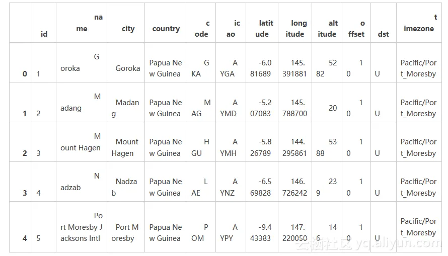
airlines.head()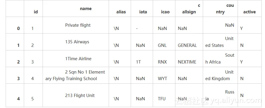
routes.head()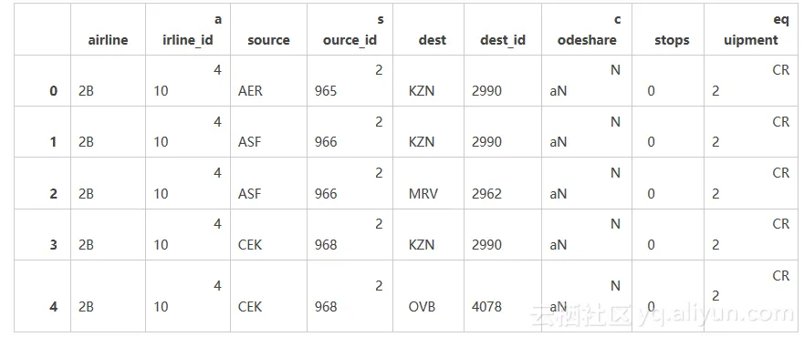
我们可以分别对每一个单独的数据集做许多不同有趣的探索,但是只要将它们结合起来分析才能取得最大的收获。Pandas 将会帮助我们分析数据,因为它能够有效的过滤权值或者通过它来应用一些函数。我们将会深入几个有趣的权值因子,比如分析航空公司和航线。
那么在此之前我们需要做一些数据清洗的工作。
routes = routes[routes["airline_id"] != "\\N"]这一行命令就确保了我们在 airline_id 这一列只含有数值型数据。
制作柱状图
现在我们理解了数据的结构,我们可以进一步地开始描点来继续探索这个问题。首先,我们将要使用 matplotlib 这个工具,matplotlib 是一个相对底层的 Python 栈中的描点库,所以它比其他的工具库要多敲一些命令来做出一个好看的曲线。另外一方面,你可以使用 matplotlib 几乎做出任何的曲线,这是因为它十分的灵活,而灵活的代价就是非常难于使用。
我们首先通过做出一个柱状图来显示不同的航空公司的航线长度分布。一个柱状图将所有的航线的长度分割到不同的值域,然后对落入到不同的值域范围内的航线进行计数。从中我们可以知道哪些航空公司的航线长,哪些航空公司的航线短。
为了达到这一点,我们需要首先计算一下航线的长度,第一步就要使用距离公式,我们将会使用余弦半正矢距离公式来计算经纬度刻画的两个点之间的距离。
import math
def haversine(lon1, lat1, lon2, lat2):
    # Convert coordinates to floats.
    lon1, lat1, lon2, lat2 = [float(lon1), float(lat1), float(lon2), float(lat2)]
    # Convert to radians from degrees.
    lon1, lat1, lon2, lat2 = map(math.radians, [lon1, lat1, lon2, lat2])
    # Compute distance.
    dlon = lon2 - lon1
    dlat = lat2 - lat1
    a = math.sin(dlat/2)**2 + math.cos(lat1) * math.cos(lat2) * math.sin(dlon/2)**2
    c = 2 * math.asin(math.sqrt(a))
    km = 6367 * c
    return km
然后我们就可以使用一个函数来计算起点机场和终点机场之间的单程距离。我们需要从路线数据框架得到机场数据框架所对应的 source_id 和 dest_id,然后与机场的数据集的 id 列相匹配,然后就只要计算就行了,这个函数是这样的:
def calc_dist(row):
    dist = 0
    try:
        # Match source and destination to get coordinates.
        source = airports[airports["id"] == row["source_id"]].iloc[0]
        dest = airports[airports["id"] == row["dest_id"]].iloc[0]
        # Use coordinates to compute distance.
        dist = haversine(dest["longitude"], dest["latitude"], source["longitude"], source["latitude"])
    except (ValueError, IndexError):
        pass
    return dist
如果 source_id 和 dest_id 列没有有效值的话,那么这个函数会报错。因此我们需要增加 try/catch 模块对这种无效的情况进行捕捉。
最后,我们将要使用 pandas 来将距离计算的函数运用到 routes 数据框架。这将会使我们得到包含所有的航线线长度的 pandas 序列,其中航线线的长度都是以公里做单位。
route_lengths = routes.apply(calc_dist, axis=1)现在我们就有了航线距离的序列了,我们将会创建一个柱状图,它将会将数据归类到对应的范围之内,然后计数分别有多少的航线落入到不同的每个范围:
import matplotlib.pyplot as plt
%matplotlib inline

plt.hist(route_lengths, bins=20)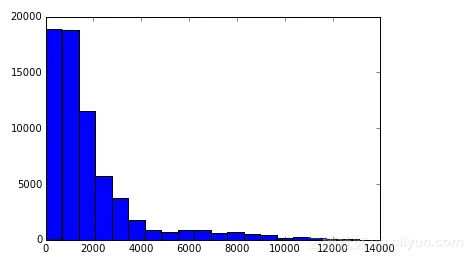
我们用 import matplotlib.pyplot as plt 导入 matplotlib 描点函数。然后我们就使用 %matplotlib inline 来设置 matplotlib 在 ipython 的 notebook 中描点,最终我们就利用 plt.hist(route_lengths, bins=20) 得到了一个柱状图。正如我们看到的,航空公司倾向于运行近距离的短程航线,而不是远距离的远程航线。
使用 seaborn
我们可以利用 seaborn 来做类似的描点,seaborn 是一个 Python 的高级库。Seaborn 建立在 matplotlib 的基础之上,做一些类型的描点,这些工作常常与简单的统计工作有关。我们可以基于一个核心的概率密度的期望,使用 distplot 函数来描绘一个柱状图。一个核心的密度期望是一个曲线 —— 本质上是一个比柱状图平滑一点的,更容易看出其中的规律的曲线。
import seaborn
seaborn.distplot(route_lengths, bins=20)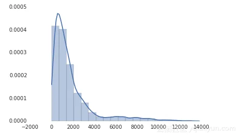
正如你所看到的那样,seaborn 同时有着更加好看的默认风格。seaborn 不含有与每个 matplotlib 的版本相对应的版本,但是它的确是一个很好的快速描点工具,而且相比于 matplotlib 的默认图表可以更好的帮助我们理解数据背后的含义。如果你想更深入的做一些统计方面的工作的话,seaborn 也不失为一个很好的库。
条形图
柱状图也虽然很好,但是有时候我们会需要航空公司的平均路线长度。这时候我们可以使用条形图--每条航线都会有一个单独的状态条,显示航空公司航线的平均长度。从中我们可以看出哪家是国内航空公司哪家是国际航空公司。我们可以使用pandas,一个python的数据分析库,来酸楚每个航空公司的平均航线长度。
import numpy
# Put relevant columns into a dataframe.
route_length_df = pandas.DataFrame({"length": route_lengths, "id": routes["airline_id"]})
# Compute the mean route length per airline.
airline_route_lengths = route_length_df.groupby("id").aggregate(numpy.mean)
# Sort by length so we can make a better chart.
airline_route_lengths = airline_route_lengths.sort("length", ascending=False)
我们首先用航线长度和航空公司的id来搭建一个新的数据框架。我们基于airline_id把route_length_df拆分成组,为每个航空公司建立一个大体的数据框架。然后我们调用pandas的aggregate函数来获取航空公司数据框架中长度列的均值,然后把每个获取到的值重组到一个新的数据模型里。之后把数据模型进行排序,这样就使得拥有最多航线的航空公司拍到了前面。
这样就可以使用matplotlib把结果画出来。
plt.bar(range(airline_route_lengths.shape[0]), airline_route_lengths["length"])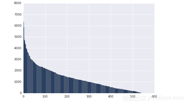
Matplotlib的plt.bar方法根据每个数据模型的航空公司平均航线长度(airline_route_lengths["length"])来做图。
问题是我们想看出哪家航空公司拥有的航线长度是什么并不容易。为了解决这个问题,我们需要能够看到坐标轴标签。这有点难,毕竟有这么多的航空公司。一个能使问题变得简单的方法是使图表具有交互性,这样能实现放大跟缩小来查看轴标签。我们可以使用bokeh库来实现这个--它能便捷的实现交互性,作出可缩放的图表。
要使用booked,我们需要先对数据进行预处理:
def lookup_name(row):
    try:
        # Match the row id to the id in the airlines dataframe so we can get the name.
        name = airlines["name"][airlines["id"] == row["id"]].iloc[0]
    except (ValueError, IndexError):
        name = ""
    return name
# Add the index (the airline ids) as a column.
airline_route_lengths["id"] = airline_route_lengths.index.copy()
# Find all the airline names.
airline_route_lengths["name"] = airline_route_lengths.apply(lookup_name, axis=1)
# Remove duplicate values in the index.
airline_route_lengths.index = range(airline_route_lengths.shape[0])
上面的代码会获取airline_route_lengths中每列的名字,然后添加到name列上,这里存贮着每个航空公司的名字。我们也添加到id列上以实现查找(apply函数不传index)。
最后,我们重置索引序列以得到所有的特殊值。没有这一步,Bokeh 无法正常运行。
现在,我们可以继续说图表问题:
import numpy as np
from bokeh.io import output_notebook
from bokeh.charts import Bar, show
output_notebook()
p = Bar(airline_route_lengths, 'name', values='length', title="Average airline route lengths")
show(p)
用 output_notebook 创建背景虚化,在 iPython 的 notebook 里画出图。然后,使用数据帧和特定序列制作条形图。最后,显示功能会显示出该图。
这个图实际上不是一个图像--它是一个 JavaScript 插件。因此,我们在下面展示的是一幅屏幕截图,而不是真实的表格。
有了它,我们可以放大,看哪一趟航班的飞行路线最长。上面的图像让这些表格看起来挤在了一起,但放大以后,看起来就方便多了。
水平条形图
Pygal 是一个能快速制作出有吸引力表格的数据分析库。我们可以用它来按长度分解路由。首先把我们的路由分成短、中、长三个距离,并在 route_lengths 里计算出它们各占的百分比。
long_routes = len([k for k in route_lengths if k > 10000]) / len(route_lengths)
medium_routes = len([k for k in route_lengths if k < 10000 and k > 2000]) / len(route_lengths)
short_routes = len([k for k in route_lengths if k < 2000]) / len(route_lengths)
然后我们可以在 Pygal 的水平条形图里把每一个都绘成条形图:
import pygal
from IPython.display import SVG
chart = pygal.HorizontalBar()
chart.title = 'Long, medium, and short routes'
chart.add('Long', long_routes * 100)
chart.add('Medium', medium_routes * 100)
chart.add('Short', short_routes * 100)
chart.render_to_file('routes.svg')
SVG(filename='routes.svg')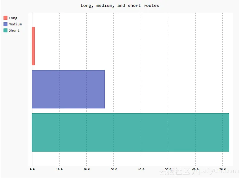
首先,我们创建一个空图。然后,我们添加元素,包括标题和条形图。每个条形图通过百分比值(最大值是100)显示出该类路由的使用频率。
最后,我们把图表渲染成文件,用 IPython 的 SVG 功能载入并展示文件。这个图看上去比默认的 matplotlib 图好多了。但是为了制作出这个图,我们要写的代码也多很多。因此,Pygal 可能比较适用于制作小型的展示用图表。
散点图
在散点图里,我们能够纵向比较数据。我们可以做一个简单的散点图来比较航空公司的 id 号和航空公司名称的长度:
name_lengths = airlines["name"].apply(lambda x: len(str(x)))
plt.scatter(airlines["id"].astype(int), name_lengths)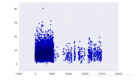
首先,我们使用 pandasapplymethod 计算每个名称的长度。它将找到每个航空公司的名字字符的数量。然后,我们使用 matplotlib 做一个散点图来比较航空 id 的长度。当我们绘制时,我们把 theidcolumn of airlines 转换为整数类型。如果我们不这样做是行不通的,因为它需要在 x 轴上的数值。我们可以看到不少的长名字都出现在早先的 id 中。这可能意味着航空公司在成立前往往有较长的名字。
我们可以使用 seaborn 验证这个直觉。Seaborn 增强版的散点图,一个联合的点,它显示了两个变量是相关的,并有着类似地分布。
data = pandas.DataFrame({"lengths": name_lengths, "ids": airlines["id"].astype(int)})
seaborn.jointplot(x="ids", y="lengths", data=data)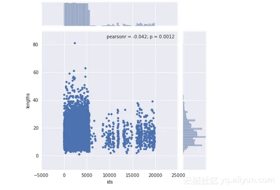
上面的图表明,两个变量之间的相关性是不明确的——r 的平方值是低的。
静态 maps
我们的数据天然的适合绘图-机场有经度和纬度对,对于出发和目的机场来说也是。
第一张图做的是显示全世界的所有机场。可以用扩展于 matplotlib 的 basemap 来做这个。这允许画世界地图和添加点,而且很容易定制。
# Import the basemap package
from mpl_toolkits.basemap import Basemap
# Create a map on which to draw.  We're using a mercator projection, and showing the whole world.
m = Basemap(projection='merc',llcrnrlat=-80,urcrnrlat=80,llcrnrlon=-180,urcrnrlon=180,lat_ts=20,resolution='c')
# Draw coastlines, and the edges of the map.
m.drawcoastlines()
m.drawmapboundary()
# Convert latitude and longitude to x and y coordinates
x, y = m(list(airports["longitude"].astype(float)), list(airports["latitude"].astype(float)))
# Use matplotlib to draw the points onto the map.
m.scatter(x,y,1,marker='o',color='red')
# Show the plot.
plt.show()
在上面的代码中,首先用 mercator projection 画一个世界地图。墨卡托投影是将整个世界的绘图投射到二位曲面。然后,在地图上用红点点画机场。
上面地图的问题是找到每个机场在哪是困难的-他们就是在机场密度高的区域合并城一团红色斑点。
就像聚焦不清楚,有个交互制图的库,folium,可以进行放大地图来帮助我们找到个别的机场。
import folium
# Get a basic world map.
airports_map = folium.Map(location=[30, 0], zoom_start=2)
# Draw markers on the map.
for name, row in airports.iterrows():
    # For some reason, this one airport causes issues with the map.
    if row["name"] != "South Pole Station":
        airports_map.circle_marker(location=[row["latitude"], row["longitude"]], popup=row["name"])
# Create and show the map.
airports_map.create_map('airports.html')
airports_map
Folium 使用 leaflet.js 来制作全交互式地图。你可以点击每一个机场在弹出框中看名字。在上边显示一个截屏,但是实际的地图更令人印象深刻。Folium 也允许非常广阔的修改选项来做更好的标注,或者添加更多的东西到地图上。
画弧线
在地图上看到所有的航空路线是很酷的,幸运的是,我们可以使用 basemap 来做这件事。我们将画弧线连接所有的机场出发地和目的地。每个弧线想展示一个段都航线的路径。不幸的是,展示所有的线路又有太多的路由,这将会是一团糟。替代,我们只现实前 3000 个路由。
# Make a base map with a mercator projection.  Draw the coastlines.
m = Basemap(projection='merc',llcrnrlat=-80,urcrnrlat=80,llcrnrlon=-180,urcrnrlon=180,lat_ts=20,resolution='c')
m.drawcoastlines()
# Iterate through the first 3000 rows.
for name, row in routes[:3000].iterrows():
    try:
        # Get the source and dest airports.
        source = airports[airports["id"] == row["source_id"]].iloc[0]
        dest = airports[airports["id"] == row["dest_id"]].iloc[0]
        # Don't draw overly long routes.
        if abs(float(source["longitude"]) - float(dest["longitude"])) < 90:
            # Draw a great circle between source and dest airports.
            m.drawgreatcircle(float(source["longitude"]), float(source["latitude"]), float(dest["longitude"]), float(dest["latitude"]),linewidth=1,color='b')
    except (ValueError, IndexError):
        pass

# Show the map.
plt.show()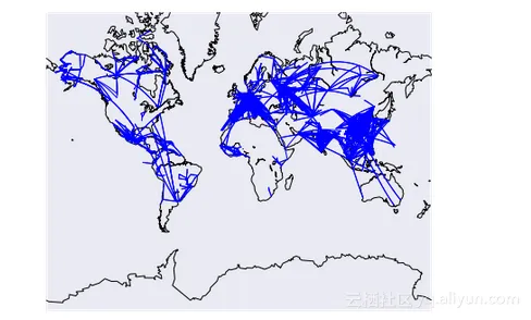
上面的代码将会画一个地图,然后再在地图上画线路。我们添加一了写过滤器来阻止过长的干扰其他路由的长路由。
画网络图
我们将做的最终的探索是画一个机场网络图。每个机场将会是网络中的一个节点,并且如果两点之间有路由将划出节点之间的连线。如果有多重路由,将添加线的权重,以显示机场连接的更多。将使用 networkx 库来做这个功能。
首先,计算机场之间连线的权重。
# Initialize the weights dictionary.
weights = {}
# Keep track of keys that have been added once -- we only want edges with a weight of more than 1 to keep our network size manageable.
added_keys = []
# Iterate through each route.
for name, row in routes.iterrows():
    # Extract the source and dest airport ids.
    source = row["source_id"]
    dest = row["dest_id"]

    # Create a key for the weights dictionary.
    # This corresponds to one edge, and has the start and end of the route.
    key = "{0}_{1}".format(source, dest)
    # If the key is already in weights, increment the weight.
    if key in weights:
        weights[key] += 1
    # If the key is in added keys, initialize the key in the weights dictionary, with a weight of 2.
    elif key in added_keys:
        weights[key] = 2
    # If the key isn't in added_keys yet, append it.
    # This ensures that we aren't adding edges with a weight of 1.
    else:
        added_keys.append(key)
一旦上面的代码运行,这个权重字典就包含了每两个机场之间权重大于或等于 2 的连线。所以任何机场有两个或者更多连接的路由将会显示出来。
# Import networkx and initialize the graph.
import networkx as nx
graph = nx.Graph()
# Keep track of added nodes in this set so we don't add twice.
nodes = set()
# Iterate through each edge.
for k, weight in weights.items():
    try:
        # Split the source and dest ids and convert to integers.
        source, dest = k.split("_")
        source, dest = [int(source), int(dest)]
        # Add the source if it isn't in the nodes.
        if source not in nodes:
            graph.add_node(source)
        # Add the dest if it isn't in the nodes.
        if dest not in nodes:
            graph.add_node(dest)
        # Add both source and dest to the nodes set.
        # Sets don't allow duplicates.
        nodes.add(source)
        nodes.add(dest)

        # Add the edge to the graph.
        graph.add_edge(source, dest, weight=weight)
    except (ValueError, IndexError):
        pass
pos=nx.spring_layout(graph)
# Draw the nodes and edges.
nx.draw_networkx_nodes(graph,pos, node_color='red', node_size=10, alpha=0.8)
nx.draw_networkx_edges(graph,pos,width=1.0,alpha=1)
# Show the plot.
plt.show()
总结
有一个成长的数据可视化的 Python 库,它可能会制作任意一种可视化。大多数库基于 matplotlib 构建的并且确保一些用例更简单。如果你想更深入的学习怎样使用 matplotlib,seaborn 和其他工具来可视化数据,在这儿检出其他课程。
文章转载自 开源中国社区[https://www.oschina.net]