💥1 概述
数据分析研究目前仍是行业热点,相关学者从数据分析关键技术中的异常检测、入侵检测、时间序列预测等角度展开研究。然而,现有研究在时间序列预测方面存在诸多局限性,没有考虑到复杂且规模庞大数据的计算消耗,忽视了非平稳数据的时间协变量漂移问题,缺乏一个实时、精准且泛化性能强的预测模型。
本文研究了使用不同的人工神经网络(即LSTM和GRU)对随机时间模型进行时间序列预测和预测的紧密程度。给定数据集包括辐照数据集和发电数据集,其基本上分别包含由传感器检测到的辐照度值和以(kw/h)为单位的发电值。
这些数据集包含从2018年12月到2019年11月的所有12个月的数据,每15分钟记录一次数据。
该项目的主要目标是找出最适合预测未来两天发电数据的ANN架构,从任何给定的一天开始,间隔为15、30、45、60分钟。
整个项目是通过matlab编程实现的。
📚2 运行结果
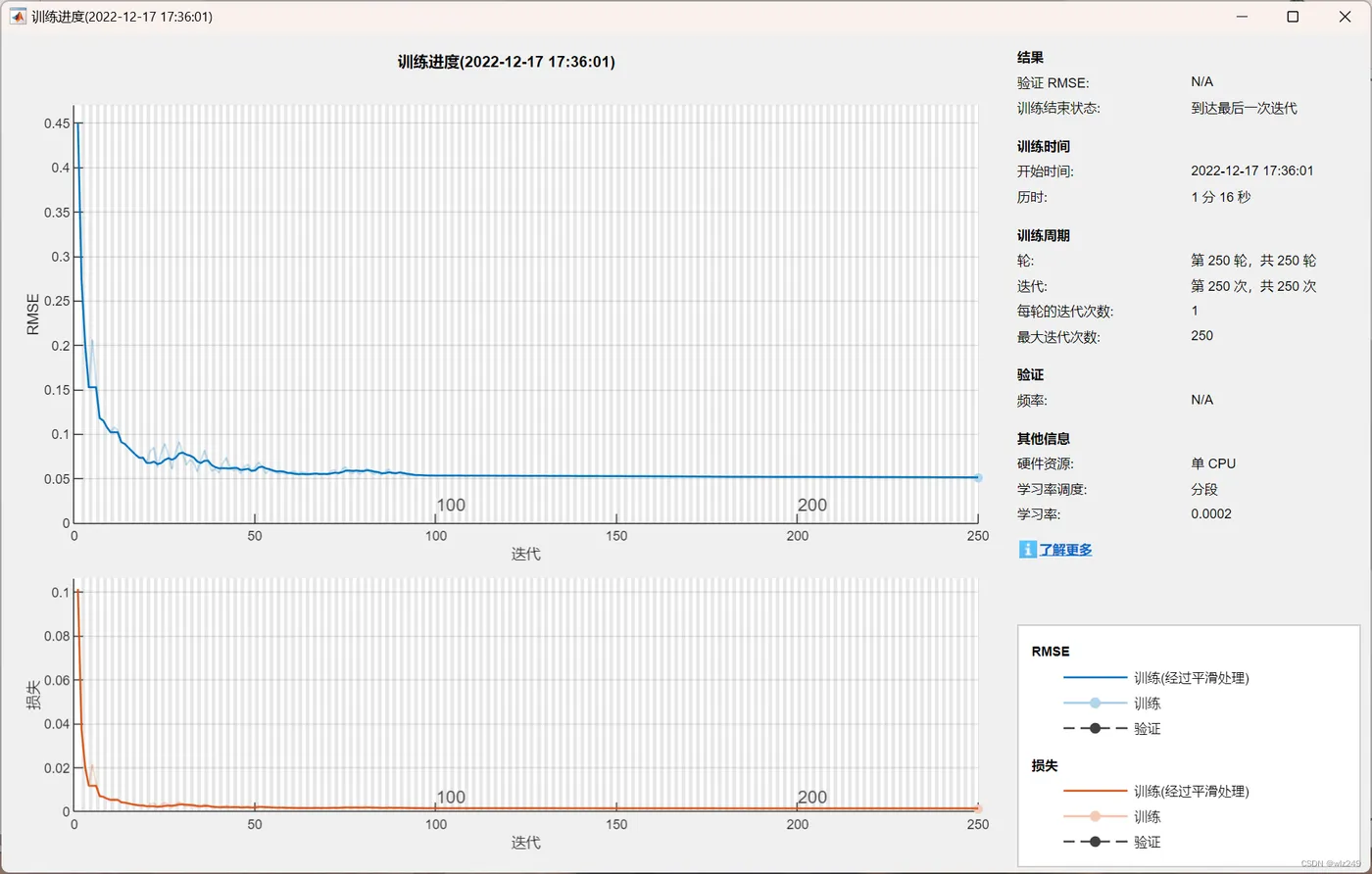
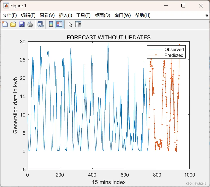
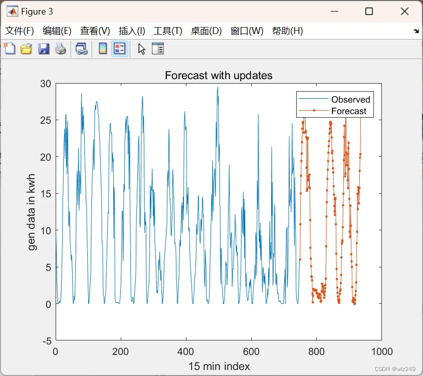
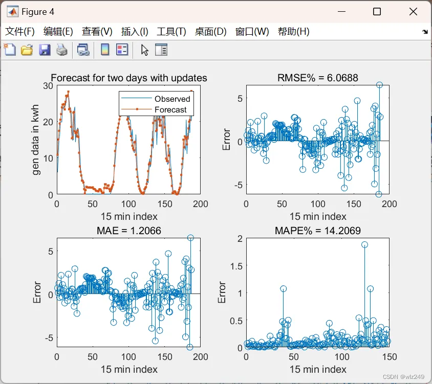
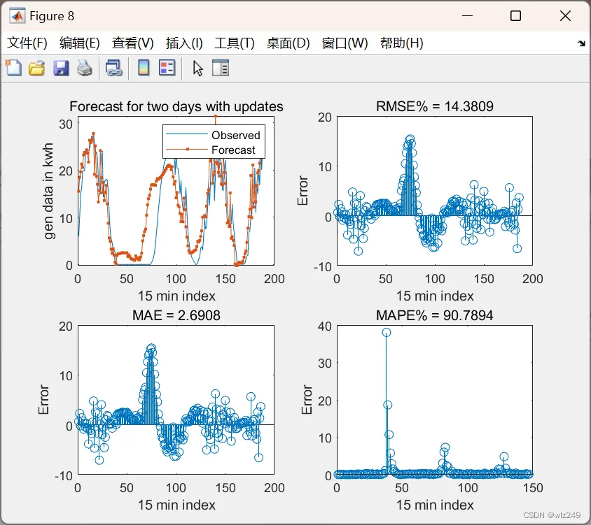
🎉3 参考文献
[1]王素. 基于深度学习的时间序列预测算法研究与应用[D].电子科技大学,2022.DOI:10.27005/d.cnki.gdzku.2022.003088.
👨💻4 Matlab代码
主函数部分代码:
load Generation_data.mat;                                                           % load data from hard drive to workspace
IrradiationData=readtable('Irradiation data.xlsx');
TrainIp=table2array(IrradiationData(1028:2927,4));                          % read data from workspace
TestIp=table2array(generationdata_table_dt(1005:2904,4));
TestIp(isnan(TrainIp)) = [];                                                % remove NAN from DATA
TrainIp(isnan(TrainIp)) = [];                                               % remove NAN from DATA
TrainIp(TestIp>50)=[];                                                      % remove noise (more than 50) from DATA
TestIp(TestIp>50)=[];                                                       % remove noise (more than 50) from DATA
TrainIp(TestIp<0)=[];                                                       % remove noise (less than 0) from DATA
TestIp(TestIp<0)=[];                                                        % remove noise (less than 0) from DATA
TestIp(TrainIp<=0)=[];                                                      % remove noise (less than 0) from DATA
TrainIp(TrainIp<=0)=[];                                                     % remove noise (less than 0) from DATA
TrainIp=TrainIp';                                                           % convert row vs column
TestIp=TestIp';
mn = min(TrainIp);                                                          % minimum of data
mx = max(TrainIp);                                                          % maximum of data
mn2 = min(TestIp);                                                          % minimum of data
mx2 = max(TestIp);                                                          % maximum of data
input = (TrainIp - mn) / (mx-mn);                                            %Normlize the Data
target = (TestIp - mn2) / (mx2-mn2);
numTimeStepsTrain = floor(0.8*numel(TrainIp));                               % 80 and 20 percent training and testing points
figure
plot(input(1:50))
hold on
plot(target(1:50),'.-')
legend(["Training" "Testing"])
xlabel("Time")
ylabel("kWh")
title(" Unit Generation")
close Figure 1;
XTrainIp = input(1:numTimeStepsTrain+1);                                     % training input data points
XTestIp = target(1:numTimeStepsTrain+1);                                     % training target data points
YTrainIp = input(numTimeStepsTrain+1:end);                                  % testing input data points
YTestIp = target(numTimeStepsTrain+1:end);
numFeatures = 2;                                                            % number of inputs=2
numResponses = 1;                                                           % number of output=1
numHiddenUnits = 200;                                                       % number of hidden unites
rmsepred=[];
rmseupdat=[];
maepred=[];
maeupdat=[];
mapepred=[];
mapeupdat=[];
layers = [ ...
    sequenceInputLayer(numFeatures)
    lstmLayer(numHiddenUnits)
    fullyConnectedLayer(numResponses)
    regressionLayer];
options = trainingOptions('adam', ...
    'MaxEpochs',250, ...
    'GradientThreshold',1, ...
    'InitialLearnRate',0.005, ...
    'MiniBatchSize',50, ...
    'LearnRateSchedule','piecewise', ...
    'LearnRateDropPeriod',90, ...
    'LearnRateDropFactor',0.2, ...
    'Verbose',false, ...
    'Plots','training-progress');                                           % LSTM other options
%     'ValidationData',{XTestIp,YTestIp},...
%     'ValidationFrequency',30, ...